This page was generated from /home/docs/checkouts/readthedocs.org/user_builds/oceanspy/checkouts/stable/docs/Tutorial.ipynb.
Tutorial
OceanSpy builds on software packages developed by the Pangeo community, in particular xarray, dask, and xgcm. It is preferable to have some familiarity with these packages to get the most out of OceanSpy.
This tutorial will take you through the main features of OceanSpy.
If you are using SciServer, make sure that you are using the Oceanography kernel. The current kernel is displayed in the top-right corner of the notebook. You can change kernel by clicking on Kernel>>Change Kernel.
To get started, import the oceanspy package:
[1]:
import oceanspy as ospy

print(ospy.__version__)
0.3.4
If you get an error that says No module named 'oceanspy', it means that you are not using the Oceanography kernel. Click on Kernel>>Change Kernel, then select Oceanography.
Dask Client
As explained here, starting a dask client is optional, but useful for optimization purposes because it provides a dashboard to monitor the computation.
On your local computer, you can access the dask dashboard just by clicking on the link displayed by the client. The dashboard link is currently not enabled on SciServer. Follow these instructions to visualize the dashboard on SciServer:
Switch to JupyterLab if you haven’t done so yet (click on
Switch To JupyterLab).Copy the link of the notebook and paste to a new tab, then substitute whatever is after the last slash with ‘dask-dashboard’.
Here is an example:
Notebook:
https://apps.sciserver.org/dockervm40/b029009b-6b4d-11e9-8a88-5254001d4703/lab?Dashboard:
https://apps.sciserver.org/dockervm40/b029009b-6b4d-11e9-8a88-5254001d4703/dask-dashboard
The link to the dashboard will be created after you execute the code below.
[2]:
from dask.distributed import Client

client = Client()
client
[2]:
Client
Client-f03afce8-d8dd-11ed-8bf7-0242ac110006
| Connection method: Cluster object | Cluster type: distributed.LocalCluster |
| Dashboard: http://127.0.0.1:8787/status |
Cluster Info
LocalCluster
a4538961
| Dashboard: http://127.0.0.1:8787/status | Workers: 4 |
| Total threads: 4 | Total memory: 100.00 GiB |
| Status: running | Using processes: True |
Scheduler Info
Scheduler
Scheduler-1a5a0e83-2549-4e24-b677-a098e4111a05
| Comm: tcp://127.0.0.1:43873 | Workers: 4 |
| Dashboard: http://127.0.0.1:8787/status | Total threads: 4 |
| Started: Just now | Total memory: 100.00 GiB |
Workers
Worker: 0
| Comm: tcp://127.0.0.1:36206 | Total threads: 1 |
| Dashboard: http://127.0.0.1:38523/status | Memory: 25.00 GiB |
| Nanny: tcp://127.0.0.1:44743 | |
| Local directory: /tmp/dask-worker-space/worker-zay_qwtp | |
Worker: 1
| Comm: tcp://127.0.0.1:32882 | Total threads: 1 |
| Dashboard: http://127.0.0.1:35209/status | Memory: 25.00 GiB |
| Nanny: tcp://127.0.0.1:40943 | |
| Local directory: /tmp/dask-worker-space/worker-rsqvgpa3 | |
Worker: 2
| Comm: tcp://127.0.0.1:37530 | Total threads: 1 |
| Dashboard: http://127.0.0.1:35630/status | Memory: 25.00 GiB |
| Nanny: tcp://127.0.0.1:35736 | |
| Local directory: /tmp/dask-worker-space/worker-dnmo4pam | |
Worker: 3
| Comm: tcp://127.0.0.1:37637 | Total threads: 1 |
| Dashboard: http://127.0.0.1:37418/status | Memory: 25.00 GiB |
| Nanny: tcp://127.0.0.1:38324 | |
| Local directory: /tmp/dask-worker-space/worker-23f7an89 | |
The client configuration can be changed and optimized for the computations needed. The main arguments to change to optimize performance are n_workers, threads_per_worker, and memory_limit.
OceanDataset
An xarray.Dataset (or ds) is the only object required to initialize an oceanspy.OceanDataset object (or od). An od is a collection of objects used by OceanSpy, and it can be initialized using the following command:
od = ospy.OceanDataset(ds)
See Import datasets for step-by-step instructions on how to import your own dataset.
Opening
Several datasets are available on SciServer (see SciServer access). Use open_oceandataset.from_catalog() to open one of these datasets (see Datasets for a list of available datasets). Otherwise, you can run this notebook on any computer by downloading the get_started data and using open_oceandataset.from_zarr().
Set SciServer = True to run this notebook on SciServer, otherwise set SciServer = False.
[3]:
SciServer = True  # True: SciServer - False: any computer
if SciServer:
    od = ospy.open_oceandataset.from_catalog("get_started")
else:
    import os

    if not os.path.isdir("oceanspy_get_started"):
        # Download get_started
        import subprocess

        print("Downloading and uncompressing get_started data...")
        print("...it might take a couple of minutes.")
        commands = [
            "wget -v -O oceanspy_get_started.tar.gz -L "
            "https://livejohnshopkins-my.sharepoint.com/"
            ":u:/g/personal/malmans2_jh_edu/"
            "EXjiMbANEHBZhy62oUDjzT4BtoJSW2W0tYtS2qO8_SM5mQ?"
            "download=1",
            "tar xvzf oceanspy_get_started.tar.gz",
            "rm -f oceanspy_get_started.tar.gz",
        ]
        subprocess.call("&&".join(commands), shell=True)
    od = ospy.open_oceandataset.from_zarr("oceanspy_get_started")

print()
print(od)
Opening get_started.
Small cutout from EGshelfIIseas2km_ASR_crop.
Citation:
 * Almansi et al., 2020 - GRL.
See also:
 * EGshelfIIseas2km_ASR_full: Full domain without variables to close budgets.
 * EGshelfIIseas2km_ASR_crop: Cropped domain with variables to close budgets.

<oceanspy.OceanDataset>

Main attributes:
   .dataset: <xarray.Dataset>
   .grid: <xgcm.Grid>
   .projection: <Projected CRS: +proj=merc +ellps=WGS84 +lon_0=0.0 +x_0=0.0 +y_0=0 ...>

More attributes:
   .name: get_started
   .description: Small cutout from EGshelfIIseas2km_ASR_crop.
   .parameters: <class 'dict'>
   .grid_coords: <class 'dict'>
Set functions
All attributes are stored as global attributes (strings) in the Dataset object, and decoded by OceanSpy. Because of this, do not change attributes directly, but use OceanSpy’s Set methods. For example:
[4]:
od = od.set_name("oceandataset #1", overwrite=True)
od = od.set_description("This is my first oceandataset", overwrite=True)
print(od)
<oceanspy.OceanDataset>

Main attributes:
   .dataset: <xarray.Dataset>
   .grid: <xgcm.Grid>
   .projection: <Projected CRS: +proj=merc +ellps=WGS84 +lon_0=0.0 +x_0=0.0 +y_0=0 ...>

More attributes:
   .name: oceandataset #1
   .description: This is my first oceandataset
   .parameters: <class 'dict'>
   .grid_coords: <class 'dict'>
The advantage of storing all the attributes in the Dataset object is that checkpoints can be created at any time (e.g., storing the Dataset in NetCDF format), and an OceanDataset object can be easily reconstructed on any computer. Thus, OceanSpy can be used at different stages of the post-processing.
Modify Dataset objects
Most OceanSpy functions modify or add variables to od.dataset. However, od.dataset is just a mirror object constructed from od._ds. If aliases have been set (this is necessary if your dataset uses variable names that differ from the OceanSpy reference names) od._ds and od.dataset differ from each other.
If you want to modify the Dataset object without using OceanSpy, you can easily extract it from od and change it using xarray. Then, you can re-initialize od if you want to use OceanSpy again. Here is an example:
[5]:
# Extract ds
ds = od.dataset

# Compute mean temperature
ds["meanTemp"] = ds["Temp"].mean("time")

# Re-initialize the OceanDataset
od = ospy.OceanDataset(ds)
print(od, "\n" * 3, od.dataset["meanTemp"])
<oceanspy.OceanDataset>

Main attributes:
   .dataset: <xarray.Dataset>
   .grid: <xgcm.Grid>
   .projection: <Projected CRS: +proj=merc +ellps=WGS84 +lon_0=0.0 +x_0=0.0 +y_0=0 ...>

More attributes:
   .name: oceandataset #1
   .description: This is my first oceandataset
   .parameters: <class 'dict'>
   .grid_coords: <class 'dict'>


 <xarray.DataArray 'meanTemp' (Z: 55, Y: 154, X: 207)>
dask.array<mean_agg-aggregate, shape=(55, 154, 207), dtype=float64, chunksize=(55, 154, 207), chunktype=numpy.ndarray>
Coordinates:
  * Z        (Z) float64 -1.0 -3.5 -7.0 -11.5 ... -681.5 -696.5 -711.5 -726.5
  * X        (X) float64 -22.02 -21.98 -21.93 -21.89 ... -13.05 -13.01 -12.96
  * Y        (Y) float64 68.99 69.01 69.03 69.04 ... 71.95 71.97 72.0 72.02
    XC       (Y, X) float64 dask.array<chunksize=(154, 207), meta=np.ndarray>
    YC       (Y, X) float64 dask.array<chunksize=(154, 207), meta=np.ndarray>
Note: Make sure that the global attributes of the Dataset do not get lost, so you will not have to re-set the attributes of the OceanDataset. Here is an example:
[6]:
import xarray as xr

# Extract ds
ds = od.dataset

# Compute mean salinity
ds = xr.merge([ds, ds["S"].mean("time").rename("meanS")])

# Global attributes have been dropped
print("Global attributes:", ds.attrs, "\n" * 2)

# Re-set global attributes
ds.attrs = od.dataset.attrs

# Re-initialize the OceanDataset
od = ospy.OceanDataset(ds)
print(od, "\n" * 3, od.dataset["meanS"])
Global attributes: {'build_date': 'ven 24 giu 2016, 09.35.54, EDT', 'build_user': 'malmans2@jhu.edu', 'MITgcm_URL': 'http://mitgcm.org', 'build_host': 'compute0117', 'MITgcm_tag_id': '1.2226 2016/01/20', 'MITgcm_version': 'checkpoint65s', 'MITgcm_mnc_ver': 0.9, 'exch2': 'True', 'OceanSpy_parameters': "{'rSphere': 6371.0, 'eq_state': 'jmd95', 'rho0': 1027, 'g': 9.81, 'eps_nh': 0, 'omega': 7.292123516990373e-05, 'c_p': 3986.0, 'tempFrz0': 0.0901, 'dTempFrz_dS': -0.0575}", 'OceanSpy_name': 'oceandataset #1', 'OceanSpy_description': 'This is my first oceandataset', 'OceanSpy_projection': 'Mercator(**{})', 'OceanSpy_grid_coords': "{'Y': {'Y': None, 'Yp1': 0.5}, 'X': {'X': None, 'Xp1': 0.5}, 'Z': {'Z': None, 'Zp1': 0.5, 'Zu': 0.5, 'Zl': -0.5}, 'time': {'time': -0.5, 'time_midp': None}}"}


<oceanspy.OceanDataset>

Main attributes:
   .dataset: <xarray.Dataset>
   .grid: <xgcm.Grid>
   .projection: <Projected CRS: +proj=merc +ellps=WGS84 +lon_0=0.0 +x_0=0.0 +y_0=0 ...>

More attributes:
   .name: oceandataset #1
   .description: This is my first oceandataset
   .parameters: <class 'dict'>
   .grid_coords: <class 'dict'>


 <xarray.DataArray 'meanS' (Z: 55, Y: 154, X: 207)>
dask.array<mean_agg-aggregate, shape=(55, 154, 207), dtype=float64, chunksize=(55, 154, 207), chunktype=numpy.ndarray>
Coordinates:
  * Z        (Z) float64 -1.0 -3.5 -7.0 -11.5 ... -681.5 -696.5 -711.5 -726.5
  * X        (X) float64 -22.02 -21.98 -21.93 -21.89 ... -13.05 -13.01 -12.96
  * Y        (Y) float64 68.99 69.01 69.03 69.04 ... 71.95 71.97 72.0 72.02
    XC       (Y, X) float64 dask.array<chunksize=(154, 207), meta=np.ndarray>
    YC       (Y, X) float64 dask.array<chunksize=(154, 207), meta=np.ndarray>
Subsampling
There are several functions that subsample the oceandataset in different ways. For example, it is possible to extract mooring sections, conduct ship surveys, or extract particle properties (see Subsampling). Most OceanSpy Computing functions make use of the xgcm functionality to have multiple axes (e.g., X and Xp1) along a single physical dimension (e.g.,
longitude). Because we will still want to be able to perform calculations on the reduced data set, the default behavior in OceanSpy is to retain all axes. The following commands extract subsets of the data and show this behavior:
[7]:
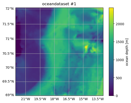
# Plot the original domain
%matplotlib inline
ax = od.plot.horizontal_section(varName="Depth")
title = ax.set_title(od.name)
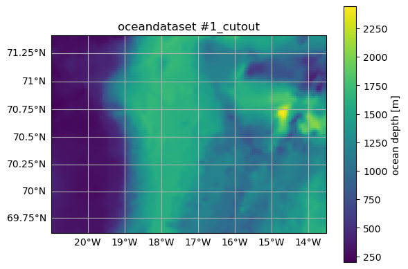
The following commands cut out and plot a small region from the original oceandataset.
[8]:
od_cut = od.subsample.cutout(
    XRange=[-21, -13.5], YRange=[69.6, 71.4], ZRange=0, timeRange="2007-09-01"
)
od_cut = od_cut.set_name("cutout", overwrite=False)
# Alternatively, this syntax can be used:
# od_cut = ospy.subsample.cutout(od, ...)

# Plot the cutout domain
ax = od_cut.plot.horizontal_section(varName="Depth")
title = ax.set_title(od_cut.name)
Cutting out the oceandataset.
The size of the dataset has been reduced, but all axes in the horizontal (X, Xp1, Y, Yp1), vertical (Z, Zp1, Zu, Zl), and time dimensions (time, time_midp) have been retained, so that od_cut is still compatible with OceanSpy:
[9]:
print("\nOriginal: {} Gigabytes".format(od.dataset.nbytes * 1.0e-9))
print(dict(od.dataset.sizes))
print("\nCutout: {} Megabytes".format(od_cut.dataset.nbytes * 1.0e-6))
print(dict(od_cut.dataset.sizes))
Original: 1.034784936 Gigabytes
{'Z': 55, 'Zp1': 56, 'Zu': 55, 'Zl': 55, 'X': 207, 'Y': 154, 'Xp1': 208, 'Yp1': 155, 'time': 4, 'time_midp': 3}

Cutout: 18.010824 Megabytes
{'Z': 1, 'Zp1': 2, 'Zu': 1, 'Zl': 1, 'X': 170, 'Y': 93, 'Xp1': 171, 'Yp1': 94, 'time': 2, 'time_midp': 1}
Sometimes it could be desirable to change this default behavior, and several additional arguments are available for this purpose (see Subsampling). For example, it is possible to reduce the vertical dimension to a single location:
[10]:
# Extract sea surface, and drop Z-axis.
od_drop = od.subsample.cutout(ZRange=0, dropAxes=True)

print("\nOriginal oceandataset:")
print(dict(od.dataset.sizes))
print(od.grid)
print("\nNew oceandataset:")
print(dict(od_drop.dataset.sizes))
print(od_drop.grid)
Cutting out the oceandataset.

Original oceandataset:
{'Z': 55, 'Zp1': 56, 'Zu': 55, 'Zl': 55, 'X': 207, 'Y': 154, 'Xp1': 208, 'Yp1': 155, 'time': 4, 'time_midp': 3}
<xgcm.Grid>
time Axis (not periodic, boundary=None):
  * center   time_midp --> outer
  * outer    time --> center
X Axis (not periodic, boundary=None):
  * center   X --> outer
  * outer    Xp1 --> center
Z Axis (not periodic, boundary=None):
  * center   Z --> left
  * outer    Zp1 --> center
  * right    Zu --> center
  * left     Zl --> center
Y Axis (not periodic, boundary=None):
  * center   Y --> outer
  * outer    Yp1 --> center

New oceandataset:
{'Z': 1, 'Zp1': 1, 'Zu': 1, 'Zl': 1, 'X': 207, 'Y': 154, 'Xp1': 208, 'Yp1': 155, 'time': 4, 'time_midp': 3}
<xgcm.Grid>
time Axis (not periodic, boundary=None):
  * center   time_midp --> outer
  * outer    time --> center
X Axis (not periodic, boundary=None):
  * center   X --> outer
  * outer    Xp1 --> center
Y Axis (not periodic, boundary=None):
  * center   Y --> outer
  * outer    Yp1 --> center
Now, the vertical dimension is no longer part of the xgcm.Grid object, and all coordinates along the vertical dimensions have size 1.
Computing
The compute module contains functions that create new variables (see Computing). Most OceanSpy functions use lazy evaluation, which means that the actual computation is not done until values are needed (e.g., when plotting). There are two different types of compute functions:
Fixed-name: Functions that do not require an input. The name of new variables is fixed.
Smart-name: Functions that do require an input (e.g., vector calculus). The name of new variables is based on input names.
Fixed-name
We compute the kinetic energy as an example. This syntax returns a dataset containing the new variable:
[11]:
ds_KE = ospy.compute.kinetic_energy(od_drop)
print(ds_KE)
Computing kinetic energy using the following parameters: {'eps_nh': 0}.
<xarray.Dataset>
Dimensions:  (Z: 1, Y: 154, time: 4, X: 207)
Coordinates:
  * Z        (Z) float64 -1.0
  * Y        (Y) float64 68.99 69.01 69.03 69.04 ... 71.95 71.97 72.0 72.02
  * time     (time) datetime64[ns] 2007-09-01 ... 2007-09-01T18:00:00
  * X        (X) float64 -22.02 -21.98 -21.93 -21.89 ... -13.05 -13.01 -12.96
Data variables:
    KE       (time, Z, Y, X) float64 dask.array<chunksize=(4, 1, 154, 207), meta=np.ndarray>
Attributes: (12/14)
    build_date:              ven 24 giu 2016, 09.35.54, EDT
    build_user:              malmans2@jhu.edu
    MITgcm_URL:              http://mitgcm.org
    build_host:              compute0117
    MITgcm_tag_id:           1.2226 2016/01/20
    MITgcm_version:          checkpoint65s
    ...                      ...
    OceanSpy_parameters:     {'rSphere': 6371.0, 'eq_state': 'jmd95', 'rho0':...
    OceanSpy_name:           oceandataset #1
    OceanSpy_description:    This is my first oceandataset
    OceanSpy_projection:     Mercator(**{})
    OceanSpy_grid_coords:    {'Y': {'Y': None, 'Yp1': 0.5}, 'X': {'X': None, ...
    OceanSpy_grid_periodic:  []
while this syntax adds the new variable to od_drop:
[12]:
od_KE = od_drop.compute.kinetic_energy()
print(od_KE.dataset)
Computing kinetic energy using the following parameters: {'eps_nh': 0}.
<xarray.Dataset>
Dimensions:     (Z: 1, Zp1: 1, Zu: 1, Zl: 1, X: 207, Y: 154, Xp1: 208,
                 Yp1: 155, time: 4, time_midp: 3)
Coordinates: (12/18)
  * Z           (Z) float64 -1.0
  * Zp1         (Zp1) float64 0.0
  * Zu          (Zu) float64 -2.0
  * Zl          (Zl) float64 0.0
  * X           (X) float64 -22.02 -21.98 -21.93 -21.89 ... -13.05 -13.01 -12.96
  * Y           (Y) float64 68.99 69.01 69.03 69.04 ... 71.95 71.97 72.0 72.02
    ...          ...
    XV          (Yp1, X) float64 dask.array<chunksize=(155, 207), meta=np.ndarray>
    YV          (Yp1, X) float64 dask.array<chunksize=(155, 207), meta=np.ndarray>
    XG          (Yp1, Xp1) float64 dask.array<chunksize=(155, 208), meta=np.ndarray>
    YG          (Yp1, Xp1) float64 dask.array<chunksize=(155, 208), meta=np.ndarray>
  * time        (time) datetime64[ns] 2007-09-01 ... 2007-09-01T18:00:00
  * time_midp   (time_midp) datetime64[ns] 2007-09-01T03:00:00 ... 2007-09-01...
Data variables: (12/88)
    drC         (Zp1) float64 dask.array<chunksize=(1,), meta=np.ndarray>
    drF         (Z) float64 dask.array<chunksize=(1,), meta=np.ndarray>
    dxC         (Y, Xp1) float64 dask.array<chunksize=(154, 208), meta=np.ndarray>
    dyC         (Yp1, X) float64 dask.array<chunksize=(155, 207), meta=np.ndarray>
    dxF         (Y, X) float64 dask.array<chunksize=(154, 207), meta=np.ndarray>
    dyF         (Y, X) float64 dask.array<chunksize=(154, 207), meta=np.ndarray>
    ...          ...
    KPPg_TH     (time_midp, Zl, Y, X) float64 dask.array<chunksize=(3, 1, 154, 207), meta=np.ndarray>
    oceQsw_AVG  (time_midp, Y, X) float64 dask.array<chunksize=(3, 154, 207), meta=np.ndarray>
    oceSPtnd    (time_midp, Z, Y, X) float64 dask.array<chunksize=(3, 1, 154, 207), meta=np.ndarray>
    meanTemp    (Z, Y, X) float64 dask.array<chunksize=(1, 154, 207), meta=np.ndarray>
    meanS       (Z, Y, X) float64 dask.array<chunksize=(1, 154, 207), meta=np.ndarray>
    KE          (time, Z, Y, X) float64 dask.array<chunksize=(4, 1, 154, 207), meta=np.ndarray>
Attributes: (12/14)
    build_date:              ven 24 giu 2016, 09.35.54, EDT
    build_user:              malmans2@jhu.edu
    MITgcm_URL:              http://mitgcm.org
    build_host:              compute0117
    MITgcm_tag_id:           1.2226 2016/01/20
    MITgcm_version:          checkpoint65s
    ...                      ...
    OceanSpy_parameters:     {'rSphere': 6371.0, 'eq_state': 'jmd95', 'rho0':...
    OceanSpy_name:           oceandataset #1
    OceanSpy_description:    This is my first oceandataset
    OceanSpy_projection:     Mercator(**{})
    OceanSpy_grid_coords:    {'Y': {'Y': None, 'Yp1': 0.5}, 'X': {'X': None, ...
    OceanSpy_grid_periodic:  []
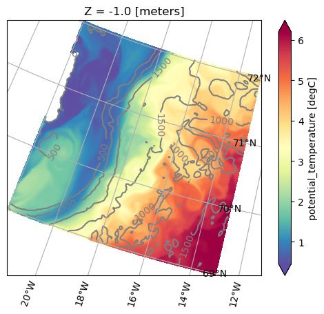
Kinetic energy has been lazily evaluated so far. We can trigger the computation by plotting the mean kinetic energy.
[13]:
od_KE.plot.horizontal_section(varName="KE", meanAxes="time")
Computing weighted_mean.
/home/idies/mambaforge/envs/Oceanography/lib/python3.9/site-packages/dask/core.py:119: RuntimeWarning: invalid value encountered in divide
  return func(*(_execute_task(a, cache) for a in args))
[13]:
<GeoAxesSubplot:title={'center':'Z = -1.0 [meters]'}, xlabel='longitude [degree_east]', ylabel='latitude [degree_north]'>
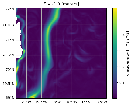
Note that OceanSpy always computes weighted means rather than regular averages!
Smart-name
We now compute gradients as an example. As seen above, od.compute.gradient(...) returns a dataset, while od = ospy.compute.gradient(od, ...) adds new variables to the oceandataset. The following cell computes temperature gradients along all dimensions:
[14]:
ds = ospy.compute.gradient(od, varNameList="Temp")
print(ds.data_vars)
Computing gradient.
Data variables:
    dTemp_dY     (time, Z, Yp1, X) float64 dask.array<chunksize=(4, 55, 155, 207), meta=np.ndarray>
    dTemp_dX     (time, Z, Y, Xp1) float64 dask.array<chunksize=(4, 55, 154, 208), meta=np.ndarray>
    dTemp_dZ     (time, Zl, Y, X) float64 dask.array<chunksize=(4, 55, 154, 207), meta=np.ndarray>
    dTemp_dtime  (time_midp, Z, Y, X) float64 dask.array<chunksize=(3, 55, 154, 207), meta=np.ndarray>
while the following code computes the temperature, salinity, and density gradients along the time dimension only. Note that Sigma0 needs to be computed.
[15]:
ds = ospy.compute.gradient(od, varNameList=["Temp", "S", "Sigma0"], axesList=["time"])
print(ds.data_vars)
Computing potential density anomaly using the following parameters: {'eq_state': 'jmd95'}.
Computing gradient.
Data variables:
    dTemp_dtime    (time_midp, Z, Y, X) float64 dask.array<chunksize=(3, 55, 154, 207), meta=np.ndarray>
    dS_dtime       (time_midp, Z, Y, X) float64 dask.array<chunksize=(3, 55, 154, 207), meta=np.ndarray>
    dSigma0_dtime  (time_midp, Z, Y, X) float64 dask.array<chunksize=(3, 55, 154, 207), meta=np.ndarray>
Here is an overview of the smart-name functions:
[16]:
print("\nGRADIENT")
print(ospy.compute.gradient(od, "Temp").data_vars)

print("\nDIVERGENCE")
print(ospy.compute.divergence(od, iName="U", jName="V", kName="W").data_vars)

print("\nCURL")
print(ospy.compute.curl(od, iName="U", jName="V", kName="W").data_vars)

print("\nLAPLACIAN")
print(ospy.compute.laplacian(od, varNameList="Temp").data_vars)

print("\nWEIGHTED MEAN")
print(ospy.compute.weighted_mean(od, varNameList="Temp").data_vars)

print("\nINTEGRAL")
print(ospy.compute.integral(od, varNameList="Temp").data_vars)
GRADIENT
Computing gradient.
Data variables:
    dTemp_dY     (time, Z, Yp1, X) float64 dask.array<chunksize=(4, 55, 155, 207), meta=np.ndarray>
    dTemp_dX     (time, Z, Y, Xp1) float64 dask.array<chunksize=(4, 55, 154, 208), meta=np.ndarray>
    dTemp_dZ     (time, Zl, Y, X) float64 dask.array<chunksize=(4, 55, 154, 207), meta=np.ndarray>
    dTemp_dtime  (time_midp, Z, Y, X) float64 dask.array<chunksize=(3, 55, 154, 207), meta=np.ndarray>

DIVERGENCE
Computing divergence.
Computing gradient.
Data variables:
    dU_dX    (time, Z, Y, X) float64 dask.array<chunksize=(4, 55, 154, 207), meta=np.ndarray>
    dV_dY    (time, Z, Y, X) float64 dask.array<chunksize=(4, 55, 154, 207), meta=np.ndarray>
    dW_dZ    (time, Z, Y, X) float64 dask.array<chunksize=(4, 55, 154, 207), meta=np.ndarray>

CURL
Computing curl.
Computing gradient.
Computing gradient.
Computing gradient.
Computing gradient.
Data variables:
    dV_dX-dU_dY  (time, Z, Yp1, Xp1) float64 dask.array<chunksize=(4, 55, 155, 208), meta=np.ndarray>
    dW_dY-dV_dZ  (time, Zl, Yp1, X) float64 dask.array<chunksize=(4, 55, 155, 207), meta=np.ndarray>
    dU_dZ-dW_dX  (time, Zl, Y, Xp1) float64 dask.array<chunksize=(4, 55, 154, 208), meta=np.ndarray>

LAPLACIAN
Computing laplacian.
Computing gradient.
Computing divergence.
Computing gradient.
Data variables:
    ddTemp_dX_dX  (time, Z, Y, X) float64 dask.array<chunksize=(4, 55, 154, 207), meta=np.ndarray>
    ddTemp_dY_dY  (time, Z, Y, X) float64 dask.array<chunksize=(4, 55, 154, 207), meta=np.ndarray>
    ddTemp_dZ_dZ  (time, Z, Y, X) float64 dask.array<chunksize=(4, 55, 154, 207), meta=np.ndarray>

WEIGHTED MEAN
Computing weighted_mean.
Data variables:
    w_mean_Temp  float64 dask.array<chunksize=(), meta=np.ndarray>
    weight_Temp  (time, Z, Y, X) float64 dask.array<chunksize=(4, 55, 154, 207), meta=np.ndarray>

INTEGRAL
Computing integral.
Data variables:
    I(Temp)dtimedXdYdZ  float64 dask.array<chunksize=(), meta=np.ndarray>
All new variables have been lazily evaluated so far. The following cell triggers the evaluation of the weighted mean temperature and salinity along all dimensions:
[17]:
ds = ospy.compute.weighted_mean(od, varNameList=["Temp", "S"], storeWeights=False)
for var in ds.data_vars:
    print("{} = {} {}".format(var, ds[var].values, ds[var].attrs.pop("units", "")))
Computing weighted_mean.
w_mean_Temp = 0.5421960292553055 degC
w_mean_S = 34.600691099468904 g kg-1
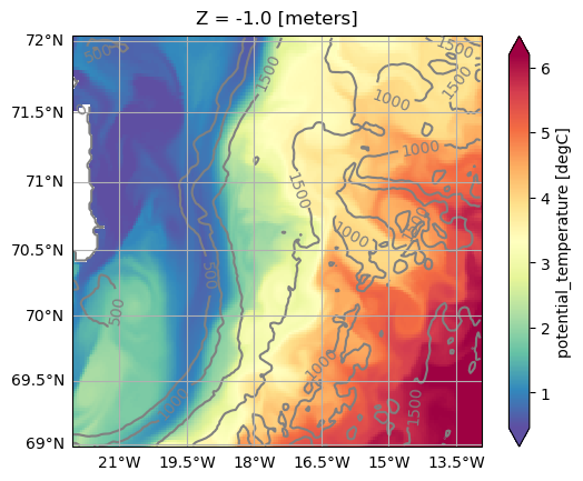
Plotting
projection of od. Here we plot the mean sea surface temperature and the isobaths using different projections:[18]:
ax = od.plot.horizontal_section(
    varName="Temp",
    contourName="Depth",
    meanAxes="time",
    center=False,
    cmap="Spectral_r",
    robust=True,
    cutout_kwargs={"ZRange": 0, "dropAxes": True},
)
Cutting out the oceandataset.
Computing weighted_mean.
Computing weighted_mean.
/home/idies/mambaforge/envs/Oceanography/lib/python3.9/site-packages/dask/core.py:119: RuntimeWarning: invalid value encountered in divide
  return func(*(_execute_task(a, cache) for a in args))
We can change the projection by using one the set functions of the Set methods of the oceandataset.
[19]:
# Change projection
od_NPS = od.set_projection("NorthPolarStereo")
ax = od_NPS.plot.horizontal_section(
    varName="Temp",
    contourName="Depth",
    meanAxes=True,
    center=False,
    cmap="Spectral_r",
    robust=True,
    cutout_kwargs={"ZRange": 0, "dropAxes": True},
)
Cutting out the oceandataset.
Computing weighted_mean.
Computing weighted_mean.
Animating
See Animating for a list of available functions. Plotting and animating functions have identical syntax. For example, just replace od.plot.horizontal_section with od.aimate.horizontal_section to create an animation of Sea Surface Temperature:
[20]:
anim = od.animate.horizontal_section(
    varName="Temp",
    contourName="Depth",
    center=False,
    cmap="Spectral_r",
    robust=True,
    cutout_kwargs={"ZRange": 0, "dropAxes": True},
    display=False,
)

# The following code is necessary to display the animation in the documentation.
# When the notebook is executed, remove the code below and set
# display=True in the command above to show the animation.
import matplotlib.pyplot as plt

dirName = "_static"
import os

try:
    os.mkdir(dirName)
except FileExistsError:
    pass
anim.save("{}/tutorial.mp4".format(dirName))
plt.close()
!ffmpeg -loglevel panic -y -i _static/tutorial.mp4 -filter_complex "[0:v] fps=12,scale=480:-1,split [a][b];[a] palettegen [p];[b][p] paletteuse" _static/tutorial.gif
!rm -f _static/tutorial.mp4
Cutting out the oceandataset.
SciServer workflow
The SciServer Interactive mode runs on a Virtual Machine with 16 cores shared between multiple users. Use it for notebooks that don’t require heavy computations, or to test and design your notebooks. Use the SciServer Jobs mode instead to fully exploit the computational power of SciServer. For larger jobs, you have exclusive access to 32 logical CPU cores and 240GiB of memory. See SciServer access for more details.
Import datasets
The following step-by-step instructions show how to import any Ocean General Circulation Model data set:
Open the dataset using
xarray. For example,
import xarray as xr
ds = open_mfdataset(paths)
Create an
OceanDataset.
import oceanspy as ospy
od = ospy.OceanDataset(ds)
- Use Set methods to connect the dataset with a
xgcm.Grid, create aliases, set parameters, …For example, setting aliases is necessary if your dataset uses variable names that differ from the OceanSpy reference names. See below for a list of OceanSpy reference names and parameters. In addition, any variable computed by OceanSpy (e.g.,Sigma0) can be aliased. Use Import methods if your dataset is not compatible with OceanSpy (e.g., remove NaNs from coordinate variables):
All commands above can be triggered using ospy.open_dataset.from_catalog and a configuration file (e.g., see SciServer catalogs).
Here we print the OceanSpy parameters that can be set.
[21]:
# Print parameters
print("\n{:>15}: {}\n".format("PARAMETER NAME", "DESCRIPTION"))
for par, desc in sorted(ospy.PARAMETERS_DESCRIPTION.items()):
    print("{:>15}: {}".format(par, desc))
 PARAMETER NAME: DESCRIPTION

            c_p: Specific heat capacity ( J/kg/K )
    dTempFrz_dS: Freezing temp. of sea water (intercept)
         eps_nh: Non-Hydrostatic coefficient.Set 0 for hydrostatic, 1 for non-hydrostatic.
       eq_state: Equation of state.
              g: Gravitational acceleration [m/s^2]
          omega: Angular velocity ( rad/s )
        rSphere: Radius of sphere for spherical polaror curvilinear grid (km).Set it None for cartesian grid.
           rho0: Reference density (Boussinesq)  ( kg/m^3 )
       tempFrz0: Freezing temp. of sea water (intercept)
While here we print the reference names of the variables used by OceanSpy.
[22]:
# Print reference names
if SciServer:
    od = ospy.open_oceandataset.from_catalog("get_started")
else:
    import os

    if not os.path.isdir("oceanspy_get_started"):
        # Download get_started
        import subprocess

        print("Downloading and uncompressing get_started data...")
        print("...it might take a couple of minutes.")
        commands = [
            "wget -v -O oceanspy_get_started.tar.gz -L "
            "https://jh.box.com/shared/static/"
            "pw83oja1gp6mbf8j34ff0qrxp08kf64q.gz",
            "tar xvzf oceanspy_get_started.tar.gz",
            "rm -f oceanspy_get_started.tar.gz",
        ]
        subprocess.call("&&".join(commands), shell=True)
    od = ospy.open_oceandataset.from_zarr("oceanspy_get_started")

table = {
    var: od.dataset[var].attrs.pop(
        "description", od.dataset[var].attrs.pop("long_name", None)
    )
    for var in od.dataset.variables
}
print("\n{:>15}: {}\n".format("REFERENCE NAME", "DESCRIPTION"))
for name, desc in sorted(table.items()):
    print("{:>15}: {}".format(name, desc))
Opening get_started.
Small cutout from EGshelfIIseas2km_ASR_crop.
Citation:
 * Almansi et al., 2020 - GRL.
See also:
 * EGshelfIIseas2km_ASR_full: Full domain without variables to close budgets.
 * EGshelfIIseas2km_ASR_crop: Cropped domain with variables to close budgets.

 REFERENCE NAME: DESCRIPTION

       ADVr_SLT: Vertical   Advective Flux of Salinity
        ADVr_TH: Vertical   Advective Flux of Pot.Temperature
       ADVx_SLT: Zonal      Advective Flux of Salinity
        ADVx_TH: Zonal      Advective Flux of Pot.Temperature
       ADVy_SLT: Meridional Advective Flux of Salinity
        ADVy_TH: Meridional Advective Flux of Pot.Temperature
       DFrI_SLT: Vertical Diffusive Flux of Salinity    (Implicit part)
        DFrI_TH: Vertical Diffusive Flux of Pot.Temperature (Implicit part)
          Depth: fluid thickness in r coordinates (at rest)
         EXFaqh: surface (2-m) specific humidity
       EXFatemp: surface (2-m) air temperature
       EXFempmr: net upward freshwater flux, > 0 increases salinity
        EXFevap: evaporation, > 0 increases salinity
          EXFhl: Latent heat flux into ocean, >0 increases theta
          EXFhs: Sensible heat flux into ocean, >0 increases theta
       EXFlwnet: Net upward longwave radiation, >0 decreases theta
       EXFpreci: precipitation, > 0 decreases salinity
       EXFpress: atmospheric pressure field
        EXFqnet: Net upward heat flux (turb+rad), >0 decreases theta
        EXFroff: river runoff, > 0 decreases salinity
        EXFroft: river runoff temperature
        EXFsnow: snow precipitation, > 0 decreases salinity
       EXFswnet: Net upward shortwave radiation, >0 decreases theta
        EXFtaux: zonal surface wind stress, >0 increases uVel
        EXFtauy: meridional surface wind stress, >0 increases vVel
       EXFuwind: zonal 10-m wind speed, >0 increases uVel
       EXFvwind: meridional 10-m wind speed, >0 increases uVel
            Eta: free-surface_r-anomaly
          HFacC: vertical fraction of open cell at cell center
          HFacS: vertical fraction of open cell at South face
          HFacW: vertical fraction of open cell at West face
       KPPg_SLT: KPP non-local Flux of Salinity
        KPPg_TH: KPP non-local Flux of Pot.Temperature
         KPPhbl: KPP boundary layer depth, bulk Ri criterion
       MXLDEPTH: Mixed-Layer Depth (>0)
       RHOAnoma: Density Anomaly (=Rho-rhoConst)
          R_low: base of fluid in r-units
        Ro_surf: surface reference (at rest) position
              S: salinity
          SFLUX: total salt flux (match salt-content variations), >0 increases salt
         SIarea: SEAICE fractional ice-covered area [0 to 1]
         SIheff: SEAICE effective ice thickness
        SIhsalt: SEAICE effective salinity
        SIhsnow: SEAICE effective snow thickness
         SIuice: SEAICE zonal ice velocity, >0 from West to East
         SIvice: SEAICE merid. ice velocity, >0 from South to North
         SRELAX: surface salinity relaxation, >0 increases salt
          TFLUX: total heat flux (match heat-content variations), >0 increases theta
         TRELAX: surface temperature relaxation, >0 increases theta
           Temp: potential_temperature
              U: Zonal Component of Velocity
              V: Meridional Component of Velocity
              W: Vertical Component of Velocity
              X: X coordinate of cell center (T-P point)
             XC: X coordinate of cell center (T-P point)
             XG: X coordinate of cell corner (Vorticity point)
             XU: X coordinate of U point
             XV: X coordinate of V point
            Xp1: X coordinate of cell corner (Vorticity point)
              Y: Y coordinate of cell center (T-P point)
             YC: Y coordinate of cell center (T-P point)
             YG: Y coordinate of cell corner (Vorticity point)
             YU: Y coordinate of U point
             YV: Y coordinate of V point
            Yp1: Y coordinate of cell corner (Vorticity point)
              Z: vertical coordinate of cell center
             Zl: vertical coordinate of upper cell interface
            Zp1: vertical coordinate of cell interface
             Zu: vertical coordinate of lower cell interface
            drC: r cell center separation
            drF: r cell face separation
            dxC: x cell center separation
            dxF: x cell face separation
            dxG: x cell corner separation
            dxV: x v-velocity separation
            dyC: y cell center separation
            dyF: y cell face separation
            dyG: y cell corner separation
            dyU: y u-velocity separation
          fCori: Coriolis f at cell center
         fCoriG: Coriolis f at cell corner
       momVort3: 3rd component (vertical) of Vorticity
       oceFWflx: net surface Fresh-Water flux into the ocean (+=down), >0 decreases salinity
       oceFreez: heating from freezing of sea-water (allowFreezing=T)
        oceQnet: net surface heat flux into the ocean (+=down), >0 increases theta
         oceQsw: net Short-Wave radiation (+=down), >0 increases theta
     oceQsw_AVG: net Short-Wave radiation (+=down), >0 increases theta
       oceSPDep: Salt plume depth based on density criterion (>0)
       oceSPflx: net surface Salt flux rejected into the ocean during freezing, (+=down),
       oceSPtnd: salt tendency due to salt plume flux >0 increases salinity
       oceSflux: net surface Salt flux into the ocean (+=down), >0 increases salinity
        oceTAUX: zonal surface wind stress, >0 increases uVel
        oceTAUY: meridional surf. wind stress, >0 increases vVel
         phiHyd: Hydrostatic Pressure Pot.(p/rho) Anomaly
      phiHydLow: Phi-Hydrostatic at r-lower boundary(bottom in z-coordinates,top in p-coordinates)
             rA: r-face area at cell center
            rAs: r-face area at V point
            rAw: r-face area at U point
            rAz: r-face area at cell corner
       surForcS: model surface forcing for Salinity, >0 increases salinity
       surForcT: model surface forcing for Temperature, >0 increases theta
           time: model_time
      time_midp: Mid-points of model_time
[ ]: