This page was generated from /home/docs/checkouts/readthedocs.org/user_builds/oceanspy/checkouts/stable/docs/Kogur.ipynb.

Use Case 1: Kögur

In this example we will subsample a dataset stored on SciServer using methods resembling field-work procedures. Specifically, we will estimate volume fluxes through the Kögur section using (i) mooring arrays, and (ii) ship surveys.

[1]:

# Import oceanspy
import cartopy.crs as ccrs

# Import additional packages used in this notebook
import matplotlib.pyplot as plt

import oceanspy as ospy

The following cell starts a dask client (see the Dask Client section in the tutorial).

[2]:

# Start client
from dask.distributed import Client

client = Client()
client

[2]:

Client

Client-1d595cc6-d8dd-11ed-8ace-0242ac110006

Connection method: Cluster object	Cluster type: distributed.LocalCluster
Dashboard: http://127.0.0.1:8787/status

Cluster Info

LocalCluster

f7012a2d

Dashboard: http://127.0.0.1:8787/status	Workers: 4
Total threads: 4	Total memory: 100.00 GiB
Status: running	Using processes: True

Scheduler Info

Scheduler

Scheduler-8b655f88-6e9c-4bdd-a062-16a2ee0522a4

Comm: tcp://127.0.0.1:39691	Workers: 4
Dashboard: http://127.0.0.1:8787/status	Total threads: 4
Started: Just now	Total memory: 100.00 GiB

Workers

Worker: 0

Comm: tcp://127.0.0.1:37895	Total threads: 1
Dashboard: http://127.0.0.1:35787/status	Memory: 25.00 GiB
Nanny: tcp://127.0.0.1:35636
Local directory: /tmp/dask-worker-space/worker-dg400ibu

Worker: 1

Comm: tcp://127.0.0.1:46138	Total threads: 1
Dashboard: http://127.0.0.1:45597/status	Memory: 25.00 GiB
Nanny: tcp://127.0.0.1:35450
Local directory: /tmp/dask-worker-space/worker-38hgqqw4

Worker: 2

Comm: tcp://127.0.0.1:33025	Total threads: 1
Dashboard: http://127.0.0.1:39132/status	Memory: 25.00 GiB
Nanny: tcp://127.0.0.1:42160
Local directory: /tmp/dask-worker-space/worker-e2fc0n1u

Worker: 3

Comm: tcp://127.0.0.1:45242	Total threads: 1
Dashboard: http://127.0.0.1:34437/status	Memory: 25.00 GiB
Nanny: tcp://127.0.0.1:36843
Local directory: /tmp/dask-worker-space/worker-8e5xgkx8

This command opens one of the datasets avaiable on SciServer.

[3]:

# Open dataset stored on SciServer.
od = ospy.open_oceandataset.from_catalog("EGshelfIIseas2km_ASR_full")

Opening EGshelfIIseas2km_ASR_full.
High-resolution (~2km) numerical simulation covering the east Greenland shelf (EGshelf),
and the Iceland and Irminger Seas (IIseas) forced by the Arctic System Reanalysis (ASR).
Citation:
 * Almansi et al., 2020 - GRL.
Characteristics:
 * full: Full domain without variables to close budgets.
See also:
 * EGshelfIIseas2km_ASR_crop: Cropped domain with variables to close budgets.

The following cell changes the default parameters used by the plotting functions.

[4]:

import matplotlib as mpl

%matplotlib inline
mpl.rcParams["figure.figsize"] = [10.0, 5.0]

Mooring array

The following diagram shows the instrumentation deployed by observational oceanographers to monitor the Kögur section (source: http://kogur.whoi.edu/img/array_boxes.png). 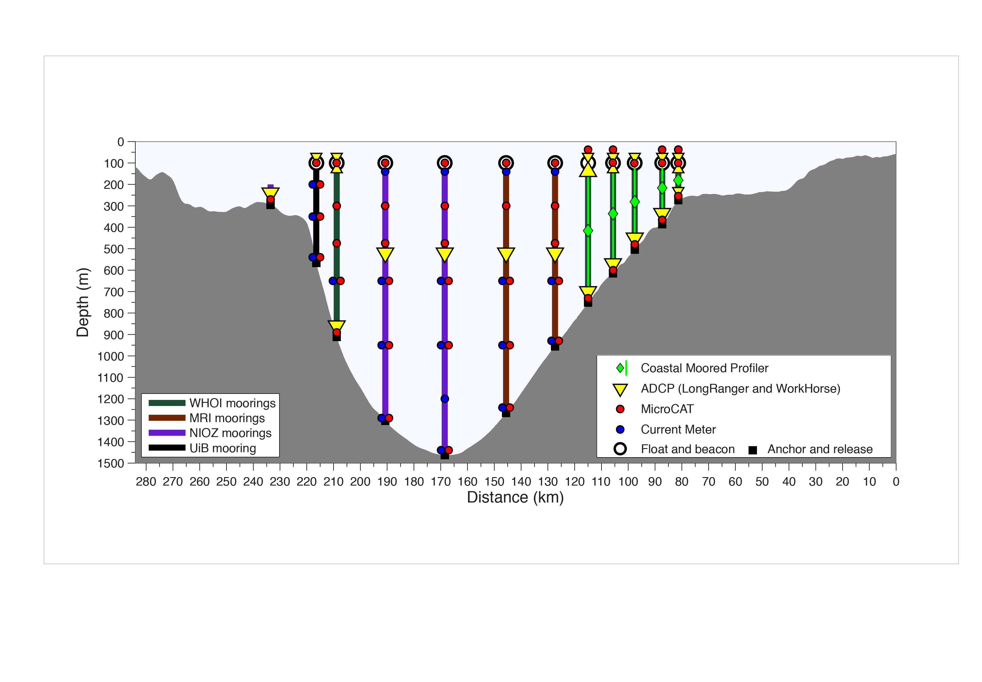Kögur Array The analogous OceanSpy function (compute.mooring_array) extracts vertical sections from the model using two criteria:

Vertical sections follow great circle paths (unless cartesian coordinates are used).
Vertical sections follow the grid of the model (extracted moorings are adjacent to each other, and the native grid of the model is preserved).

[5]:

# Kögur information
lats_Kogur = [68.68, 67.52, 66.49]
lons_Kogur = [-26.28, -23.77, -22.99]
depth_Kogur = [0, -1750]

# Select time range:
# September 2007, extracting one snapshot every 3 days
timeRange = ["2007-09-01", "2007-09-30T18"]
timeFreq = "3D"

# Extract mooring array and fields used by this notebook
od_moor = od.subsample.mooring_array(
    Xmoor=lons_Kogur,
    Ymoor=lats_Kogur,
    ZRange=depth_Kogur,
    timeRange=timeRange,
    timeFreq=timeFreq,
    varList=["Temp", "S", "U", "V", "dyG", "dxG", "drF", "HFacS", "HFacW"],
)

Cutting out the oceandataset.

/home/idies/mambaforge/envs/Oceanography/lib/python3.9/site-packages/oceanspy/subsample.py:1375: UserWarning:
Time resampling drops variables on `time_midp` dimension.
Dropped variables: ['time_midp'].
  return cutout(self._od, **kwargs)
/home/idies/mambaforge/envs/Oceanography/lib/python3.9/site-packages/dask/array/core.py:1712: FutureWarning: The `numpy.column_stack` function is not implemented by Dask array. You may want to use the da.map_blocks function or something similar to silence this warning. Your code may stop working in a future release.
  warnings.warn(

Extracting mooring array.

The following cell shows how to store the mooring array in a NetCDF file. In this use case, we only use this feature to create a checkpoint. Another option could be to move the file to other servers or computers. If the NetCDF is re-opened using OceanSpy (as shown below), all OceanSpy functions are enabled and can be applied to the oceandataset.

[6]:

# Store the new mooring dataset
filename = "Kogur_mooring.nc"
od_moor.to_netcdf(filename)

# The NetCDF can now be re-opened with oceanspy at any time,
# and on any computer
od_moor = ospy.open_oceandataset.from_netcdf(filename)

# Print size
print("Size:")
print(" * Original dataset: {0:.1f} TB".format(od.dataset.nbytes * 1.0e-12))
print(" * Mooring dataset: {0:.1f} MB".format(od_moor.dataset.nbytes * 1.0e-6))
print()

Writing dataset to [Kogur_mooring.nc].
Opening dataset from [Kogur_mooring.nc].
Size:
 * Original dataset: 17.5 TB
 * Mooring dataset: 12.1 MB

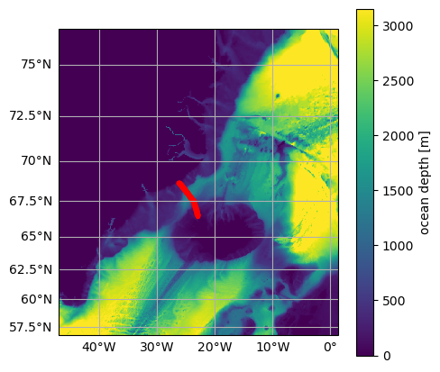
The following map shows the location of the moorings forming the Kögur section.

[7]:

# Plot map and mooring locations
fig = plt.figure(figsize=(5, 5))
ax = od.plot.horizontal_section(varName="Depth")
XC = od_moor.dataset["XC"].squeeze()
YC = od_moor.dataset["YC"].squeeze()
line = ax.plot(XC, YC, "r.", transform=ccrs.PlateCarree())

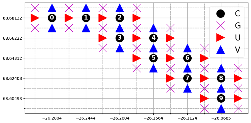
The following figure shows the grid structure of the mooring array. The original grid structure of the model is unchaged, and each mooring is associated with one C-gridpoint (e.g., hydrography), two U-gridpoint and two V-gridpoint (e.g., velocities), and four G-gripoint (e.g., vertical component of relative vorticity).

[8]:

# Print grid
print(od_moor.grid)
print()
print(od_moor.dataset.coords)
print()

# Plot 10 moorings and their grid points
fig, ax = plt.subplots(1, 1)
n_moorings = 10
# Markers:
for _, (pos, mark, col) in enumerate(
    zip(["C", "G", "U", "V"], ["o", "x", ">", "^"], ["k", "m", "r", "b"])
):
    X = od_moor.dataset["X" + pos].values[:n_moorings].flatten()
    Y = od_moor.dataset["Y" + pos].values[:n_moorings].flatten()
    ax.plot(X, Y, col + mark, markersize=20, label=pos)
    if pos == "C":
        for i in range(n_moorings):
            ax.annotate(
                str(i),
                (X[i], Y[i]),
                size=15,
                weight="bold",
                color="w",
                ha="center",
                va="center",
            )
        ax.set_xticks(X, minor=False)
        ax.set_yticks(Y, minor=False)
    elif pos == "G":
        ax.set_xticks(X, minor=True)
        ax.set_yticks(Y, minor=True)
ax.legend(prop={"size": 20})
ax.grid(which="major", linestyle="-")
ax.grid(which="minor", linestyle="--")

<xgcm.Grid>
mooring Axis (not periodic, boundary=None):
  * center   mooring_midp --> outer
  * outer    mooring --> center
time Axis (not periodic, boundary=None):
  * center   time_midp --> outer
  * outer    time --> center
Z Axis (not periodic, boundary=None):
  * center   Z --> left
  * outer    Zp1 --> center
  * right    Zu --> center
  * left     Zl --> center
Y Axis (not periodic, boundary=None):
  * center   Y --> outer
  * outer    Yp1 --> center
X Axis (not periodic, boundary=None):
  * center   X --> outer
  * outer    Xp1 --> center

Coordinates:
  * Z                  (Z) float64 -1.0 -3.5 -7.0 ... -1.732e+03 -1.746e+03
  * Zp1                (Zp1) float64 0.0 -2.0 -5.0 ... -1.739e+03 -1.754e+03
  * Zu                 (Zu) float64 -2.0 -5.0 -9.0 ... -1.739e+03 -1.754e+03
  * Zl                 (Zl) float64 0.0 -2.0 -5.0 ... -1.724e+03 -1.739e+03
    YC                 (mooring, Y, X) float64 ...
    Xind               (mooring, Y, X) float64 ...
    Yind               (mooring, Y, X) float64 ...
  * mooring            (mooring) int64 0 1 2 3 4 5 6 ... 185 186 187 188 189 190
  * Y                  (Y) int64 0
  * X                  (X) int64 0
    XC                 (mooring, Y, X) float64 ...
    YU                 (mooring, Y, Xp1) float64 ...
  * Xp1                (Xp1) int64 0 1
    XU                 (mooring, Y, Xp1) float64 ...
    YV                 (mooring, Yp1, X) float64 ...
  * Yp1                (Yp1) int64 0 1
    XV                 (mooring, Yp1, X) float64 ...
    YG                 (mooring, Yp1, Xp1) float64 ...
    XG                 (mooring, Yp1, Xp1) float64 ...
  * time               (time) datetime64[ns] 2007-09-01 ... 2007-09-28
  * time_midp          (time_midp) datetime64[ns] 2007-09-02T12:00:00 ... 200...
    mooring_dist       (mooring) float64 ...
  * mooring_midp       (mooring_midp) float64 0.5 1.5 2.5 ... 187.5 188.5 189.5
    mooring_midp_dist  (mooring_midp) float64 ...

Plots

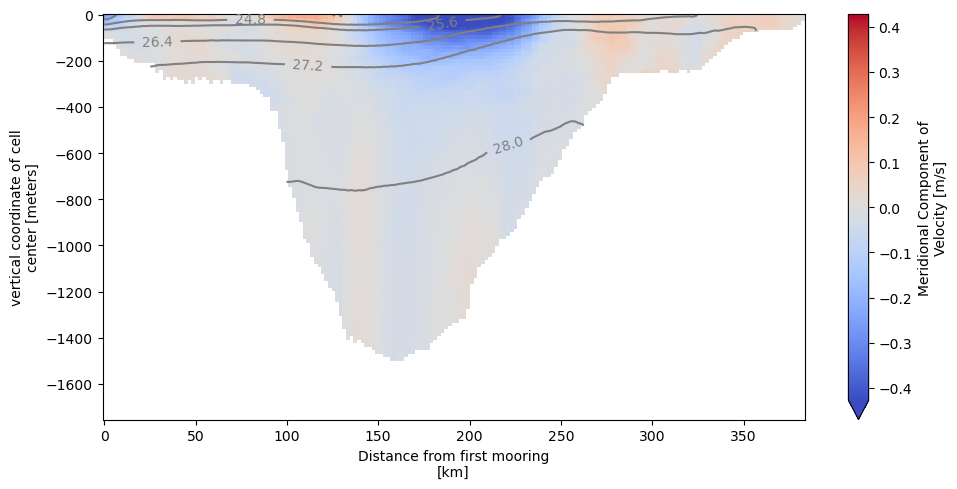
Vertical sections

We can now use OceanSpy to plot vertical sections. Here we plot isopycnal contours on top of the mean meridional velocities (V). Although there are two V-points associated with each mooring, the plot can be displayed because OceanSpy automatically performs a linear interpolation using the grid object.

[9]:

# Plot time mean
ax = od_moor.plot.vertical_section(
    varName="V",
    contourName="Sigma0",
    meanAxes="time",
    robust=True,
    cmap="coolwarm",
)

Computing potential density anomaly using the following parameters: {'eq_state': 'jmd95'}.
Computing weighted_mean.
Regridding [w_mean_V] along [Y]-axis.
Computing weighted_mean.

It is possible to visualize all the snapshots by omitting the meanAxes='time' argument:

[10]:

# Plot all snapshots
ax = od_moor.plot.vertical_section(
    varName="V", contourName="Sigma0", robust=True, cmap="coolwarm", col_wrap=5
)
# Alternatively, use the following command to produce a movie:
# anim = od_moor.animate.vertical_section(varName='V', contourName='Sigma0', ...)

Computing potential density anomaly using the following parameters: {'eq_state': 'jmd95'}.
Regridding [V] along [Y]-axis.

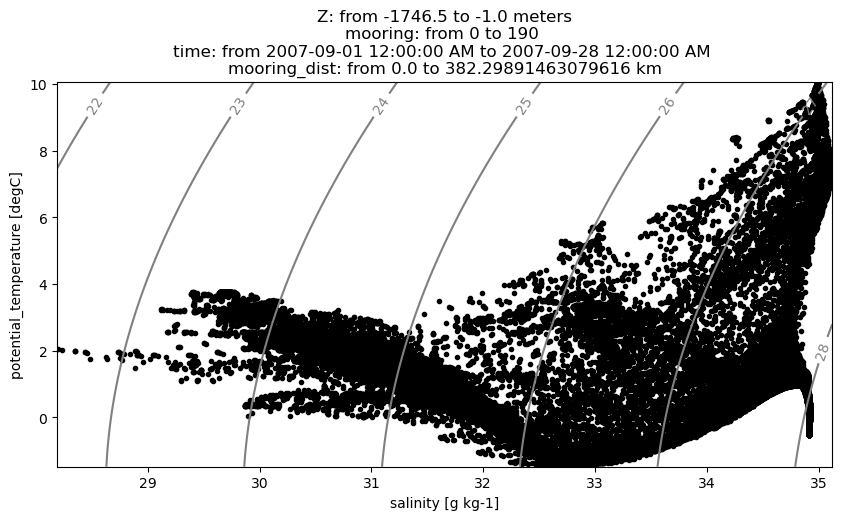
TS-diagrams

Here we use OceanSpy to plot a Temperature-Salinity diagram.

[11]:

ax = od_moor.plot.TS_diagram()
# Alternatively, use the following command
# to explore how the water masses change with time:
# anim = od_moor.animate.TS_diagram()

Isopycnals: Computing potential density anomaly using the following parameters: {'eq_state': 'jmd95'}.

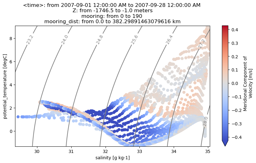
We can also color each TS point using any field in the original dataset, or any field computed by OceanSpy. Fields that are not on the same grid of temperature and salinity are automatically regridded by OceanSpy.

[12]:

ax = od_moor.plot.TS_diagram(
    colorName="V",
    meanAxes="time",
    cmap_kwargs={"robust": True, "cmap": "coolwarm"},
)

Computing weighted_mean.
Computing weighted_mean.
Interpolating [V] along [Y]-axis.
Isopycnals: Computing potential density anomaly using the following parameters: {'eq_state': 'jmd95'}.

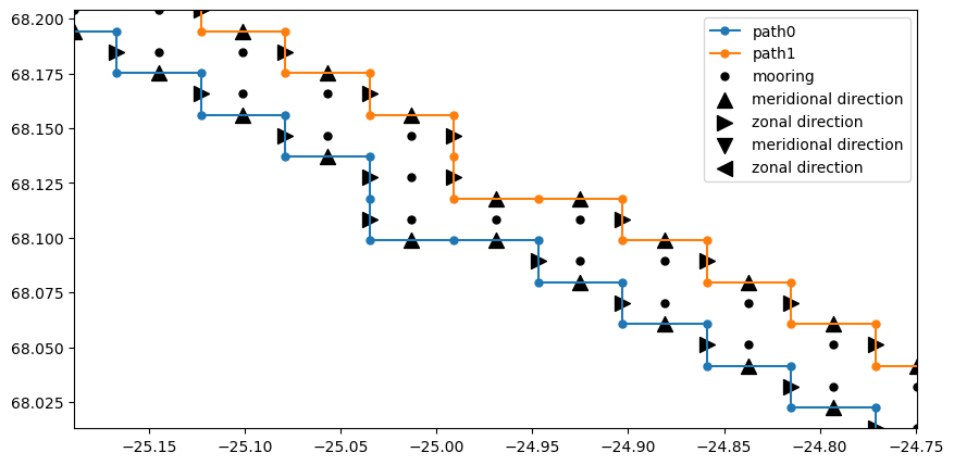
Volume flux

OceanSpy can be used to compute accurate volume fluxes through vertical sections. The function compute.mooring_volume_transport calculates the inflow/outflow through all grid faces of the vertical section. This function creates a new dimension named path because transports can be computed using two paths (see the plot below).

[13]:

# Show volume flux variables
ds_Vflux = ospy.compute.mooring_volume_transport(od_moor)
od_moor = od_moor.merge_into_oceandataset(ds_Vflux)
print(ds_Vflux)

# Plot 10 moorings and volume flux directions.
fig, ax = plt.subplots(1, 1)
ms = 10
s = 100
ds = od_moor.dataset
_ = ax.step(
    ds["XU"].isel(Xp1=0).squeeze().values,
    ds["YV"].isel(Yp1=0).squeeze().values,
    "C0.-",
    ms=ms,
    label="path0",
)
_ = ax.step(
    ds["XU"].isel(Xp1=1).squeeze().values,
    ds["YV"].isel(Yp1=1).squeeze().values,
    "C1.-",
    ms=ms,
    label="path1",
)
_ = ax.plot(ds["XC"].squeeze(), ds["YC"].squeeze(), "k.", ms=ms, label="mooring")
_ = ax.scatter(
    ds["X_Vtransport"].where(ds["dir_Vtransport"] == 1),
    ds["Y_Vtransport"].where(ds["dir_Vtransport"] == 1),
    s=s,
    c="k",
    marker="^",
    label="meridional direction",
)
_ = ax.scatter(
    ds["X_Utransport"].where(ds["dir_Utransport"] == 1),
    ds["Y_Utransport"].where(ds["dir_Utransport"] == 1),
    s=s,
    c="k",
    marker=">",
    label="zonal direction",
)
_ = ax.scatter(
    ds["X_Vtransport"].where(ds["dir_Vtransport"] == -1),
    ds["Y_Vtransport"].where(ds["dir_Vtransport"] == -1),
    s=s,
    c="k",
    marker="v",
    label="meridional direction",
)
_ = ax.scatter(
    ds["X_Utransport"].where(ds["dir_Utransport"] == -1),
    ds["Y_Utransport"].where(ds["dir_Utransport"] == -1),
    s=s,
    c="k",
    marker="<",
    label="zonal direction",
)
# Only show a few moorings
m_start = 50
m_end = 70
xlim = ax.set_xlim(
    sorted(
        [
            ds["XC"].isel(mooring=m_start).values,
            ds["XC"].isel(mooring=m_end).values,
        ]
    )
)
ylim = ax.set_ylim(
    sorted(
        [
            ds["YC"].isel(mooring=m_start).values,
            ds["YC"].isel(mooring=m_end).values,
        ]
    )
)
ax.legend()

Computing horizontal volume transport.
<xarray.Dataset>
Dimensions:         (Z: 123, mooring: 191, time: 10, path: 2)
Coordinates: (12/13)
  * Z               (Z) float64 -1.0 -3.5 -7.0 ... -1.732e+03 -1.746e+03
  * mooring         (mooring) int64 0 1 2 3 4 5 6 ... 185 186 187 188 189 190
    Y               int64 0
    YU              (mooring) float64 68.68 68.68 68.68 ... 66.52 66.5 66.49
  * time            (time) datetime64[ns] 2007-09-01 2007-09-04 ... 2007-09-28
    mooring_dist    (mooring) float64 0.0 1.778 3.556 ... 378.1 380.2 382.3
    ...              ...
    X               int64 0
    XV              (mooring) float64 -26.29 -26.24 -26.2 ... -22.99 -22.99
    YC              (mooring) float64 68.68 68.68 68.68 ... 66.52 66.5 66.49
    Xind            (mooring) float64 -26.29 -26.24 -26.2 ... -22.99 -22.99
    Yind            (mooring) float64 68.68 68.68 68.68 ... 66.52 66.5 66.49
    XC              (mooring) float64 -26.29 -26.24 -26.2 ... -22.99 -22.99
Data variables:
    transport       (time, Z, mooring, path) float64 nan nan ... nan nan
    Vtransport      (time, Z, mooring, path) float64 nan nan ... nan nan
    Utransport      (time, Z, mooring, path) float64 nan nan -0.0 ... nan nan
    Y_transport     (mooring) float64 ...
    X_transport     (mooring) float64 ...
    Y_Utransport    (mooring, path) float64 68.68 68.68 nan ... 66.5 66.49 66.49
    X_Utransport    (mooring, path) float64 -26.31 -26.31 nan ... -23.01 -23.01
    Y_Vtransport    (mooring, path) float64 68.67 68.67 68.69 ... 66.48 66.48
    X_Vtransport    (mooring, path) float64 -26.29 -26.29 ... -22.99 -22.99
    dir_Utransport  (mooring, path) float64 nan nan nan nan ... 1.0 1.0 nan nan
    dir_Vtransport  (mooring, path) float64 nan nan 1.0 1.0 ... nan nan nan nan
Attributes: (12/14)
    build_date:              ven 24 giu 2016, 09.35.54, EDT
    build_user:              malmans2@jhu.edu
    MITgcm_URL:              http://mitgcm.org
    build_host:              compute0117
    MITgcm_tag_id:           1.2226 2016/01/20
    MITgcm_version:          checkpoint65s
    ...                      ...
    OceanSpy_parameters:     {'rSphere': 6371.0, 'eq_state': 'jmd95', 'rho0':...
    OceanSpy_name:           EGshelfIIseas2km_ASR_full
    OceanSpy_description:    High-resolution (~2km) numerical simulation cove...
    OceanSpy_projection:     Mercator(**{})
    OceanSpy_grid_coords:    {'Y': {'Y': None, 'Yp1': 0.5}, 'X': {'X': None, ...
    OceanSpy_grid_periodic:  []

[13]:

<matplotlib.legend.Legend at 0x7f09c607c280>

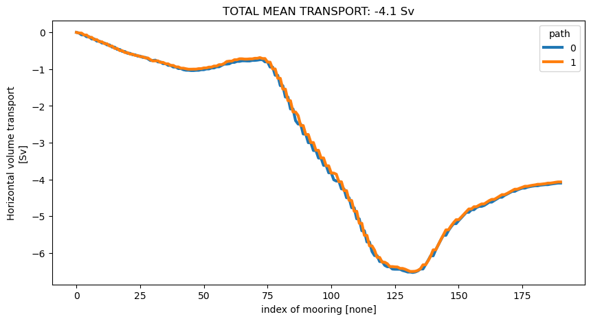
Here we compute and plot the cumulative mean transport through the Kögur mooring array.

[14]:

# Compute cumulative transport
tran_moor = od_moor.dataset["transport"]
cum_tran_moor = tran_moor.sum("Z").mean("time").cumsum("mooring")
cum_tran_moor.attrs = tran_moor.attrs
fig, ax = plt.subplots(1, 1)
lines = cum_tran_moor.squeeze().plot.line(hue="path", linewidth=3)
tot_mean_tran_moor = cum_tran_moor.isel(mooring=-1).mean("path")
title = ax.set_title(
    "TOTAL MEAN TRANSPORT: {0:.1f} Sv" "".format(tot_mean_tran_moor.values)
)

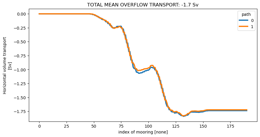
Here we compute the transport of the overflow, defined as water with density greater than 27.8 kg m\(^{-3}\).

[15]:

# Mask transport using density
od_moor = od_moor.compute.potential_density_anomaly()
density = od_moor.dataset["Sigma0"].squeeze()
oflow_moor = tran_moor.where(density > 27.8)

# Compute cumulative transport as before
cum_oflow_moor = oflow_moor.sum("Z").mean("time").cumsum("mooring")
cum_oflow_moor.attrs = oflow_moor.attrs
fig, ax = plt.subplots(1, 1)
lines = cum_oflow_moor.squeeze().plot.line(hue="path", linewidth=3)
tot_mean_oflow_moor = cum_oflow_moor.isel(mooring=-1).mean("path")
title = ax.set_title(
    "TOTAL MEAN OVERFLOW TRANSPORT: {0:.1f} Sv" "".format(tot_mean_oflow_moor.values)
)

Computing potential density anomaly using the following parameters: {'eq_state': 'jmd95'}.

Ship survey

The following picture shows the NATO Research Vessel Alliance, a ship designed to carry out research at sea (source: http://www.marina.difesa.it/noi-siamo-la-marina/mezzi/forze-navali/PublishingImages/_alliance.jpg). Survey ship

The OceanSpy function analogous to a ship survey (compute.survey_stations) extracts vertical sections from the model using two criteria:

Vertical sections follow great circle paths (unless cartesian coordinates are used) with constant horizontal spacing between stations.
Interpolation is performed and all fields are returned at the same locations (the native grid of the model is NOT preserved).

[16]:

# Spacing between interpolated stations
delta_Kogur = 2  # km

# Extract survey stations
# Reduce dataset to speed things up:
od_surv = od.subsample.survey_stations(
    Xsurv=lons_Kogur,
    Ysurv=lats_Kogur,
    delta=delta_Kogur,
    ZRange=depth_Kogur,
    timeRange=timeRange,
    timeFreq=timeFreq,
    varList=["Temp", "S", "U", "V", "drC", "drF", "HFacC", "HFacW", "HFacS"],
)

Cutting out the oceandataset.

/home/idies/mambaforge/envs/Oceanography/lib/python3.9/site-packages/oceanspy/subsample.py:1375: UserWarning:
Time resampling drops variables on `time_midp` dimension.
Dropped variables: ['time_midp'].
  return cutout(self._od, **kwargs)

Carrying out survey.
Variables to interpolate: ['XC', 'YC', 'XU', 'YU', 'XV', 'YV', 'XG', 'YG', 'HFacC', 'HFacW', 'HFacS', 'U', 'V', 'Temp', 'S', 'Xind', 'Yind'].
Interpolating [XC].
Interpolating [YC].
Interpolating [XU].
Interpolating [YU].
Interpolating [XV].
Interpolating [YV].
Interpolating [XG].
Interpolating [YG].
Interpolating [HFacC].
Interpolating [HFacW].
Interpolating [HFacS].
Interpolating [U].
Interpolating [V].
Interpolating [Temp].
Interpolating [S].
Interpolating [Xind].

/home/idies/mambaforge/envs/Oceanography/lib/python3.9/site-packages/xesmf/smm.py:130: UserWarning: Input array is not C_CONTIGUOUS. Will affect performance.
  warnings.warn('Input array is not C_CONTIGUOUS. ' 'Will affect performance.')

Interpolating [Yind].

/home/idies/mambaforge/envs/Oceanography/lib/python3.9/site-packages/xesmf/smm.py:130: UserWarning: Input array is not C_CONTIGUOUS. Will affect performance.
  warnings.warn('Input array is not C_CONTIGUOUS. ' 'Will affect performance.')

[17]:

# Plot map and survey stations
fig = plt.figure(figsize=(5, 5))
ax = od.plot.horizontal_section(varName="Depth")
XC = od_surv.dataset["XC"].squeeze()
YC = od_surv.dataset["YC"].squeeze()
line = ax.plot(XC, YC, "r.", transform=ccrs.PlateCarree())

Orthogonal velocities

We can use OceanSpy to compute the velocity components orthogonal and tangential to the Kögur section.

[18]:

od_surv = od_surv.compute.survey_aligned_velocities()

Computing survey aligned velocities.

/home/idies/mambaforge/envs/Oceanography/lib/python3.9/site-packages/oceanspy/compute.py:3002: UserWarning:
These variables are not available and can not be computed: ['AngleCS', 'AngleSN'].
If you think that OceanSpy should be able to compute them, please open an issue on GitHub:
 https://github.com/hainegroup/oceanspy/issues
Assuming U=U_zonal and V=V_merid.
If you are using curvilinear coordinates, run `compute.geographical_aligned_velocities` before `subsample.survey_stations`
  ds = survey_aligned_velocities(self._od, **kwargs)

The following animation shows isopycnal contours on top of the velocity component orthogonal to the Kögur section.

[19]:

anim = od_surv.animate.vertical_section(
    varName="ort_Vel",
    contourName="Sigma0",
    robust=True,
    cmap="coolwarm",
    display=False,
)

# The following code is necessary to display the animation in the documentation.
# When the notebook is executed, remove the code below and set
# display=True in the command above to show the animation.
import matplotlib.pyplot as plt

dirName = "_static"
import os

try:
    os.mkdir(dirName)
except FileExistsError:
    pass
anim.save("{}/Kogur.mp4".format(dirName))
plt.close()
!ffmpeg -loglevel panic -y -i _static/Kogur.mp4 -filter_complex "[0:v] fps=12,scale=480:-1,split [a][b];[a] palettegen [p];[b][p] paletteuse" _static/Kogur.gif
!rm -f _static/Kogur.mp4

Finally, we can infer the volume flux by integrating the orthogonal velocities.

[20]:

# Integrate along Z
od_surv = od_surv.compute.integral(varNameList="ort_Vel", axesList=["Z"])
# Compute transport using weights
od_surv = od_surv.compute.weighted_mean(
    varNameList="I(ort_Vel)dZ", axesList=["station"]
)
transport_surv = (
    od_surv.dataset["I(ort_Vel)dZ"] * od_surv.dataset["weight_I(ort_Vel)dZ"]
)
# Convert in Sverdrup
transport_surv = transport_surv * 1.0e-6
# Compute cumulative transport
cum_transport_surv = transport_surv.cumsum("station").rename(
    "Horizontal volume transport"
)
cum_transport_surv.attrs["units"] = "Sv"

Computing integral.
Computing weighted_mean.

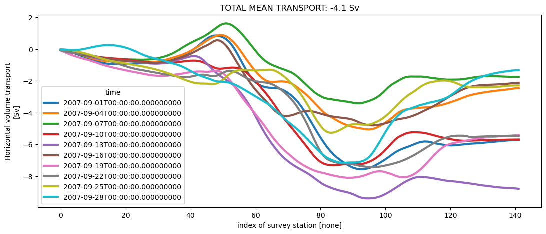
Here we plot the cumulative transport for each snapshot.

[21]:

# Plot
fig, ax = plt.subplots(figsize=(13, 5))
lines = cum_transport_surv.squeeze().plot.line(hue="time", linewidth=3)
tot_mean_transport = cum_transport_surv.isel(station=-1).mean("time")
title = ax.set_title(
    "TOTAL MEAN TRANSPORT: {0:.1f} Sv".format(tot_mean_transport.values)
)