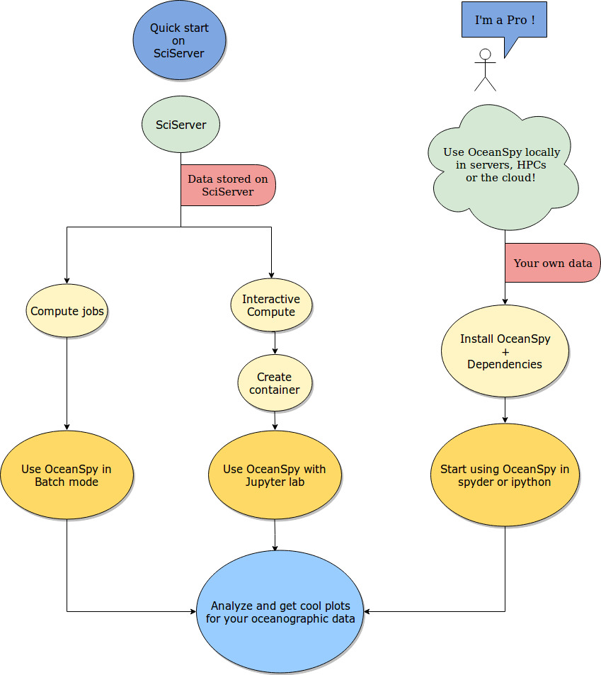
Quick Start
Click on the following badge to run the notebook immediately: ![]()
The badge above opens the tutorial notebook in an executable environment without any dataset. Follow the instructions below to learn how to use OceanSpy with the Datasets on the Johns Hopkins University SciServer system.
OceanSpy and its dependencies are preinstalled on SciServer. There is no need to download and install it unless you wish to run OceanSpy on your local machine or server. Steps to do that are described in the Installation section.
The following steps explain how to navigate through the basics of OceanSpy on SciServer. Steps 1 to 5 describe how to create a container on SciServer with a set of example datasets to work on.
Go to www.sciserver.org.
Log in or create a new account.
Click on
Compute.Click on
Create container, then use the following settings:Domain:
Interactive Docker Compute Domain
Compute Image:
Oceanography
User volumes:
persistent
scratch
Data volumes:
Ocean Circulation
Click on
Create.
Steps 6 to 8 describe how to get started with using the container. Information about which directories to work in and their descriptions are detailed below the container images once they are created on SciServer.
Click on the name of the new container.
Click on
Storage>>your_username>>persistent.Click on
New>>Oceanography.
Steps 9 to 15 demonstrate a subset of the commonly used OceanSpy commands.
Copy and paste the following lines in the first notebook cell to import OceanSpy, and open the get started dataset:
import oceanspy as ospy
od = ospy.open_oceandataset.from_catalog('get_started')
Use the following line to extract a limited geographic range of the dataset:
od_cutout = od.subsample.cutout(YRange=[69.6, 71.4], XRange=[-21, -15], ZRange=[0, -100])
Use the following line to plot a map of weighted mean temperature:
ax = od_cutout.plot.horizontal_section(varName='Temp', meanAxes=['Z', 'time'], center=False)
Use the following line to compute the potential density anomaly:
od_cutout = od_cutout.compute.potential_density_anomaly()
Use the following line to store the cutout in netCDF format:
od_cutout.to_netcdf('filename.nc')
The netCDF file can be download and used for post-processing offline, or kept on SciServer. Any software of choice can be used to re-open the netCDF file. To re-open the file using OceanSpy, use the following command:
od_cutout = ospy.open_oceandataset.from_netcdf('filename.nc')
Opening the netCDF file using OceanSpy will allows the use of OceanSpy’s functions whether it be on SciServer or a local machine. For example, the following line plots an animated TS diagram color-coded by potential density anomaly (computed in step 12):
anim = od_cutout.animate.TS_diagram(colorName='Sigma0', meanAxes='Z')
The get_started is just a small cutout from a high-resolution realistic dataset. Click Datasets for a list of datasets available on SciServer.
Check out Tutorial, Use Cases, and API reference to learn more about OceanSpy and its features, and feel free to open an issue here, or to send an email to mattia.almansi@noc.ac.uk if you have any questions.
Interactive Demo
You can interactively explore many more features at www.bndr.it/gfvgd
The schematic below shows how OceanSpy is designed to be used by the oceanographic community.