This page was generated from /home/docs/checkouts/readthedocs.org/user_builds/oceanspy/checkouts/latest/docs/Particles.ipynb.
Use Case 2: Particles
In this example we will subsample a dataset stored on SciServer using trajectories of synthetic Lagrangian particles. OceanSpy enables the extraction of properties at any given location, but it does not have functionality to compute Lagrangian trajectories yet. The trajectories used in this notebook have been previously computed using a Matlab-based Lagrangian particle code (Gelderloos et al., 2016). The Lagrangian particle code, along with synthetic oceanographic observational platforms (such as Argo floats, isobaric floats, current profiler, and gliders), will be incorporated into OceanSpy in future releases.
The animation below shows the change in temperature of synthetic particles along their 3D trajectories. Particles have been released in Denmark Strait and tracked backward in time from day 0 to day 180, and tracked forward in time from day 180 to 360. All particles are animated forward in time. Source: https://player.vimeo.com/video/296949375
[1]:
# Display animation
from IPython.display import HTML

# Link
s = "https://player.vimeo.com/video/296949375"

# Options
w = 640
h = 360
f = 0
a = "autoplay; fullscreen"

# Display
HTML(
    f'<iframe src="{s}"'
    'width="640" height="360" frameborder="0" allow="autoplay; fullscreen"'
    "allowfullscreen></iframe>"
)
/home/idies/mambaforge/envs/Oceanography/lib/python3.9/site-packages/IPython/core/display.py:431: UserWarning: Consider using IPython.display.IFrame instead
  warnings.warn("Consider using IPython.display.IFrame instead")
[1]:
Extract
The computational time to extract particle properties depends on the number of particles, the length of their trajectories, the number of variables requested, and, more importantly, how far the particles travel in the domain and therefore, how dispersed the Lagrangian trajectories are. Thus, it is preferable to extract particle properties asynchronously using the Job mode of SciServer compute (see SciServer access for step-by-step instructions). This
notebook, when executed in interactive mode, skips the subsampling step. Instead, it loads an OceanDataset previously created executing the same notebook in Job mode.
Set interactive = True to run in Interactive mode, or interactive = False to run in Job mode. Alternatively, you can activate the Job mode by typing interactive = False in the Parameters slot of the SciServer Job submission form.
[2]:
interactive = True  # True: Interactive - False: Job

# Check parameters.txt
try:
    # Use values from parameters.txt
    f = open("parameters.txt", "r")
    for line in f:
        exec(line)
    f.close()
except FileNotFoundError:
    # Keep preset values
    pass
The following cell starts a dask client (see the Dask Client section in the tutorial).
[3]:
# Start Client
from dask.distributed import Client

client = Client()
client
[3]:
Client
Client-ac9f71bc-d8db-11ed-8a48-0242ac110006
| Connection method: Cluster object | Cluster type: distributed.LocalCluster |
| Dashboard: http://127.0.0.1:8787/status |
Cluster Info
LocalCluster
fd40e064
| Dashboard: http://127.0.0.1:8787/status | Workers: 4 |
| Total threads: 4 | Total memory: 100.00 GiB |
| Status: running | Using processes: True |
Scheduler Info
Scheduler
Scheduler-ba5c5b4a-57ca-450f-a56f-6a9529bc98c5
| Comm: tcp://127.0.0.1:40685 | Workers: 4 |
| Dashboard: http://127.0.0.1:8787/status | Total threads: 4 |
| Started: Just now | Total memory: 100.00 GiB |
Workers
Worker: 0
| Comm: tcp://127.0.0.1:37562 | Total threads: 1 |
| Dashboard: http://127.0.0.1:39030/status | Memory: 25.00 GiB |
| Nanny: tcp://127.0.0.1:44469 | |
| Local directory: /tmp/dask-worker-space/worker-5eczcgfc | |
Worker: 1
| Comm: tcp://127.0.0.1:40873 | Total threads: 1 |
| Dashboard: http://127.0.0.1:38400/status | Memory: 25.00 GiB |
| Nanny: tcp://127.0.0.1:34121 | |
| Local directory: /tmp/dask-worker-space/worker-0p2ot6wv | |
Worker: 2
| Comm: tcp://127.0.0.1:33771 | Total threads: 1 |
| Dashboard: http://127.0.0.1:36647/status | Memory: 25.00 GiB |
| Nanny: tcp://127.0.0.1:33261 | |
| Local directory: /tmp/dask-worker-space/worker-og03lnsb | |
Worker: 3
| Comm: tcp://127.0.0.1:40242 | Total threads: 1 |
| Dashboard: http://127.0.0.1:41705/status | Memory: 25.00 GiB |
| Nanny: tcp://127.0.0.1:38136 | |
| Local directory: /tmp/dask-worker-space/worker-8yonp5i0 | |
While the following cell set up the environment.
[4]:
import matplotlib.pyplot as plt
import numpy as np

# Additional imports
import xarray as xr
from cartopy.crs import PlateCarree

# Import OceanSpy
import oceanspy as ospy
Here we open the OceanDataset containing the Eulerian fields that we want to sample along the Lagrangian trajectories. Then, for plotting purposes, we mask out the land from the bathymetry (variable Depth) and merge the variable masked_Depth into the OceanDataset.
[5]:
# Open OceanDataset (eulerian fields)
od_eul = ospy.open_oceandataset.from_catalog("EGshelfIIseas2km_ASR_full")

# Mask depth for plotting purposes
Depth = od_eul.dataset["Depth"]
Depth = Depth.where(Depth > 0)
od_eul = od_eul.merge_into_oceandataset(Depth.rename("masked_Depth"))
Opening EGshelfIIseas2km_ASR_full.
High-resolution (~2km) numerical simulation covering the east Greenland shelf (EGshelf),
and the Iceland and Irminger Seas (IIseas) forced by the Arctic System Reanalysis (ASR).
Citation:
 * Almansi et al., 2020 - GRL.
Characteristics:
 * full: Full domain without variables to close budgets.
See also:
 * EGshelfIIseas2km_ASR_crop: Cropped domain with variables to close budgets.
We will analyze about 4,000 synthetic particles released in Denmark Strait at the end of February, and tracked forward in time for 30 days (with 6 hour resolution). The following properties will be extracted: temperature, salinity, ocean depth, and the vertical component of relative vorticity. Note that OceanSpy can extract any property, and variables such as momVort3 that are not in the model cell centers can be subsampled.
[6]:
import os
import subprocess

# Create or download OceanDataset with particle properties
mat_name = "oceanspy_particle_trajectories.mat"  # Used by Job
nc_name = "oceanspy_particle_properties.nc"  # Created by Job
if interactive:
    # Download OceanDataset
    if not os.path.isdir(mat_name):
        import subprocess

        print(f"Downloading [{nc_name}].")
        commands = [
            f"wget -v -O {nc_name} -L "
            "https://livejohnshopkins-my.sharepoint.com/"
            ":u:/g/personal/malmans2_jh_edu/"
            "EWvf_TyoEdpaDKcFacaPLI4B1fLGf9qleW7xbIDlKVPJDw?"
            "download=1"
        ]
        subprocess.call("&&".join(commands), shell=True)
else:
    # Download trajectories
    if not os.path.isdir(mat_name):
        print(f"Downloading [{mat_name}].")
        commands = [
            f"wget -v -O {mat_name} -L "
            "https://livejohnshopkins-my.sharepoint.com/"
            ":u:/g/personal/malmans2_jh_edu/"
            "ETSRG8OcbWpccc7zx_rbzsIBqBl1UATQSwNTjqtk9fLR-Q?"
            "download=1"
        ]
        subprocess.call("&&".join(commands), shell=True)

    # Read trajectories
    import scipy.io as sio

    particle_data = sio.loadmat(mat_name)

    # Get time
    time_origin = np.datetime64("2008-02-29T00:00")
    times = np.asarray(
        [
            time_origin + np.timedelta64(int(dt * 24), "h")
            for dt in particle_data["timee"].squeeze()
        ]
    )

    # Get trajectories
    Xpart = particle_data["f_lons"].transpose()
    Ypart = particle_data["f_lats"].transpose()
    Zpart = particle_data["f_deps"].transpose()

    # Pick variables (velocities and hydrography)
    varList = ["Temp", "S", "momVort3", "Depth"]

    # Extract properties
    od_lag = ospy.subsample.particle_properties(
        od_eul,
        times=times,
        Ypart=Ypart,
        Xpart=Xpart,
        Zpart=Zpart,
        varList=varList,
    )

    # Save in netCDF format
    od_lag.to_netcdf(nc_name)

# Open OceanDataset
od_lag = ospy.open_oceandataset.from_netcdf(nc_name)
Downloading [oceanspy_particle_properties.nc].
--2023-04-11 22:44:06--  https://livejohnshopkins-my.sharepoint.com/:u:/g/personal/malmans2_jh_edu/EWvf_TyoEdpaDKcFacaPLI4B1fLGf9qleW7xbIDlKVPJDw?download=1
Resolving livejohnshopkins-my.sharepoint.com (livejohnshopkins-my.sharepoint.com)... 13.107.138.8, 13.107.136.8, 2620:1ec:8f8::8, ...
Connecting to livejohnshopkins-my.sharepoint.com (livejohnshopkins-my.sharepoint.com)|13.107.138.8|:443... connected.
HTTP request sent, awaiting response... 302 Found
Location: /personal/malmans2_jh_edu/Documents/BoxMigration/oceanspy_particle_properties.nc?ga=1 [following]
--2023-04-11 22:44:07--  https://livejohnshopkins-my.sharepoint.com/personal/malmans2_jh_edu/Documents/BoxMigration/oceanspy_particle_properties.nc?ga=1
Reusing existing connection to livejohnshopkins-my.sharepoint.com:443.
HTTP request sent, awaiting response... 200 OK
Length: 45981653 (44M) [application/x-netcdf]
Saving to: ‘oceanspy_particle_properties.nc’

     0K .......... .......... .......... .......... ..........  0%  166K 4m31s
    50K .......... .......... .......... .......... ..........  0% 6.05M 2m19s
   100K .......... .......... .......... .......... ..........  0% 11.6M 94s
   150K .......... .......... .......... .......... ..........  0% 6.16M 72s
   200K .......... .......... .......... .......... ..........  0% 5.79M 59s
   250K .......... .......... .......... .......... ..........  0% 6.10M 50s
   300K .......... .......... .......... .......... ..........  0% 11.4M 44s
   350K .......... .......... .......... .......... ..........  0% 2.57M 40s
   400K .......... .......... .......... .......... ..........  1% 6.13M 37s
   450K .......... .......... .......... .......... ..........  1% 10.5M 33s
   500K .......... .......... .......... .......... ..........  1% 5.65M 31s
   550K .......... .......... .......... .......... ..........  1% 10.0M 29s
   600K .......... .......... .......... .......... ..........  1% 5.55M 27s
   650K .......... .......... .......... .......... ..........  1% 10.4M 25s
   700K .......... .......... .......... .......... ..........  1% 5.71M 24s
   750K .......... .......... .......... .......... ..........  1% 11.1M 23s
   800K .......... .......... .......... .......... ..........  1% 10.5M 22s
   850K .......... .......... .......... .......... ..........  2% 9.71M 21s
   900K .......... .......... .......... .......... ..........  2% 6.04M 20s
   950K .......... .......... .......... .......... ..........  2% 11.8M 19s
  1000K .......... .......... .......... .......... ..........  2% 12.0M 18s
  1050K .......... .......... .......... .......... ..........  2%  306K 24s
  1100K .......... .......... .......... .......... ..........  2% 11.7M 23s
  1150K .......... .......... .......... .......... ..........  2%  144K 35s
  1200K .......... .......... .......... .......... ..........  2% 4.04M 34s
  1250K .......... .......... .......... .......... ..........  2% 5.90M 33s
  1300K .......... .......... .......... .......... ..........  3% 5.87M 32s
  1350K .......... .......... .......... .......... ..........  3% 4.12M 31s
  1400K .......... .......... .......... .......... ..........  3% 6.07M 30s
  1450K .......... .......... .......... .......... ..........  3% 3.64M 29s
  1500K .......... .......... .......... .......... ..........  3% 5.98M 29s
  1550K .......... .......... .......... .......... ..........  3% 5.83M 28s
  1600K .......... .......... .......... .......... ..........  3% 5.93M 27s
  1650K .......... .......... .......... .......... ..........  3% 5.94M 27s
  1700K .......... .......... .......... .......... ..........  3% 6.18M 26s
  1750K .......... .......... .......... .......... ..........  4% 11.1M 25s
  1800K .......... .......... .......... .......... ..........  4% 6.26M 25s
  1850K .......... .......... .......... .......... ..........  4% 6.10M 24s
  1900K .......... .......... .......... .......... ..........  4% 11.6M 24s
  1950K .......... .......... .......... .......... ..........  4% 6.08M 23s
  2000K .......... .......... .......... .......... ..........  4% 11.5M 23s
  2050K .......... .......... .......... .......... ..........  4% 11.6M 22s
  2100K .......... .......... .......... .......... ..........  4% 5.73M 22s
  2150K .......... .......... .......... .......... ..........  4% 11.1M 22s
  2200K .......... .......... .......... .......... ..........  5% 12.1M 21s
  2250K .......... .......... .......... .......... ..........  5% 5.99M 21s
  2300K .......... .......... .......... .......... ..........  5% 11.2M 20s
  2350K .......... .......... .......... .......... ..........  5% 11.7M 20s
  2400K .......... .......... .......... .......... ..........  5% 12.2M 20s
  2450K .......... .......... .......... .......... ..........  5% 11.2M 19s
  2500K .......... .......... .......... .......... ..........  5% 10.7M 19s
  2550K .......... .......... .......... .......... ..........  5% 11.3M 19s
  2600K .......... .......... .......... .......... ..........  5% 12.0M 18s
  2650K .......... .......... .......... .......... ..........  6% 11.3M 18s
  2700K .......... .......... .......... .......... ..........  6% 12.1M 18s
  2750K .......... .......... .......... .......... ..........  6% 11.9M 18s
  2800K .......... .......... .......... .......... ..........  6% 11.7M 17s
  2850K .......... .......... .......... .......... ..........  6% 11.8M 17s
  2900K .......... .......... .......... .......... ..........  6% 12.0M 17s
  2950K .......... .......... .......... .......... ..........  6% 12.2M 17s
  3000K .......... .......... .......... .......... ..........  6% 11.7M 16s
  3050K .......... .......... .......... .......... ..........  6% 11.3M 16s
  3100K .......... .......... .......... .......... ..........  7% 12.7M 16s
  3150K .......... .......... .......... .......... ..........  7% 12.1M 16s
  3200K .......... .......... .......... .......... ..........  7% 12.2M 15s
  3250K .......... .......... .......... .......... ..........  7% 13.0M 15s
  3300K .......... .......... .......... .......... ..........  7% 10.9M 15s
  3350K .......... .......... .......... .......... ..........  7% 49.5M 15s
  3400K .......... .......... .......... .......... ..........  7%  255K 17s
  3450K .......... .......... .......... .......... ..........  7% 29.7K 37s
  3500K .......... .......... .......... .......... ..........  7% 45.3K 49s
  3550K .......... .......... .......... .......... ..........  8% 74.0K 56s
  3600K .......... .......... .......... .......... ..........  8% 1.50M 55s
  3650K .......... .......... .......... .......... ..........  8% 2.35M 55s
  3700K .......... .......... .......... .......... ..........  8% 3.82M 54s
  3750K .......... .......... .......... .......... ..........  8% 5.64M 53s
  3800K .......... .......... .......... .......... ..........  8% 5.78M 53s
  3850K .......... .......... .......... .......... ..........  8% 5.67M 52s
  3900K .......... .......... .......... .......... ..........  8% 11.1M 52s
  3950K .......... .......... .......... .......... ..........  8% 10.8M 51s
  4000K .......... .......... .......... .......... ..........  9% 11.7M 50s
  4050K .......... .......... .......... .......... ..........  9% 11.1M 50s
  4100K .......... .......... .......... .......... ..........  9% 11.7M 49s
  4150K .......... .......... .......... .......... ..........  9% 12.0M 48s
  4200K .......... .......... .......... .......... ..........  9% 11.5M 48s
  4250K .......... .......... .......... .......... ..........  9% 10.8M 47s
  4300K .......... .......... .......... .......... ..........  9% 11.7M 47s
  4350K .......... .......... .......... .......... ..........  9% 11.8M 46s
  4400K .......... .......... .......... .......... ..........  9% 11.6M 46s
  4450K .......... .......... .......... .......... .......... 10% 12.2M 45s
  4500K .......... .......... .......... .......... .......... 10% 11.9M 45s
  4550K .......... .......... .......... .......... .......... 10% 12.4M 44s
  4600K .......... .......... .......... .......... .......... 10% 11.4M 44s
  4650K .......... .......... .......... .......... .......... 10% 12.2M 43s
  4700K .......... .......... .......... .......... .......... 10% 12.0M 43s
  4750K .......... .......... .......... .......... .......... 10% 57.2M 42s
  4800K .......... .......... .......... .......... .......... 10% 12.4M 42s
  4850K .......... .......... .......... .......... .......... 10% 11.7M 41s
  4900K .......... .......... .......... .......... .......... 11% 11.7M 41s
  4950K .......... .......... .......... .......... .......... 11% 12.5M 40s
  5000K .......... .......... .......... .......... .......... 11% 66.5M 40s
  5050K .......... .......... .......... .......... .......... 11% 12.2M 39s
  5100K .......... .......... .......... .......... .......... 11% 12.6M 39s
  5150K .......... .......... .......... .......... .......... 11% 12.6M 39s
  5200K .......... .......... .......... .......... .......... 11% 12.2M 38s
  5250K .......... .......... .......... .......... .......... 11% 59.9M 38s
  5300K .......... .......... .......... .......... .......... 11% 13.1M 38s
  5350K .......... .......... .......... .......... .......... 12%  304K 38s
  5400K .......... .......... .......... .......... .......... 12% 6.14M 38s
  5450K .......... .......... .......... .......... .......... 12% 38.5K 47s
  5500K .......... .......... .......... .......... .......... 12%  123K 49s
  5550K .......... .......... .......... .......... .......... 12%  107K 52s
  5600K .......... .......... .......... .......... .......... 12% 42.5K 60s
  5650K .......... .......... .......... .......... .......... 12% 31.4K 70s
  5700K .......... .......... .......... .......... .......... 12%  195K 71s
  5750K .......... .......... .......... .......... .......... 12% 1.36M 71s
  5800K .......... .......... .......... .......... .......... 13% 3.86M 70s
  5850K .......... .......... .......... .......... .......... 13% 2.88M 69s
  5900K .......... .......... .......... .......... .......... 13% 10.9M 69s
  5950K .......... .......... .......... .......... .......... 13% 5.83M 68s
  6000K .......... .......... .......... .......... .......... 13% 11.4M 68s
  6050K .......... .......... .......... .......... .......... 13% 11.2M 67s
  6100K .......... .......... .......... .......... .......... 13% 11.4M 66s
  6150K .......... .......... .......... .......... .......... 13% 12.0M 66s
  6200K .......... .......... .......... .......... .......... 13% 77.7M 65s
  6250K .......... .......... .......... .......... .......... 14% 11.6M 65s
  6300K .......... .......... .......... .......... .......... 14% 11.8M 64s
  6350K .......... .......... .......... .......... .......... 14% 12.7M 63s
  6400K .......... .......... .......... .......... .......... 14% 11.9M 63s
  6450K .......... .......... .......... .......... .......... 14% 65.4M 62s
  6500K .......... .......... .......... .......... .......... 14% 12.1M 62s
  6550K .......... .......... .......... .......... .......... 14% 13.5M 61s
  6600K .......... .......... .......... .......... .......... 14% 4.41M 61s
  6650K .......... .......... .......... .......... .......... 14% 12.5M 60s
  6700K .......... .......... .......... .......... .......... 15% 80.1M 60s
  6750K .......... .......... .......... .......... .......... 15% 12.3M 59s
  6800K .......... .......... .......... .......... .......... 15% 14.3M 59s
  6850K .......... .......... .......... .......... .......... 15% 21.1M 58s
  6900K .......... .......... .......... .......... .......... 15% 21.2M 58s
  6950K .......... .......... .......... .......... .......... 15% 13.6M 57s
  7000K .......... .......... .......... .......... .......... 15% 4.47M 57s
  7050K .......... .......... .......... .......... .......... 15% 12.2M 56s
  7100K .......... .......... .......... .......... .......... 15% 82.3M 56s
  7150K .......... .......... .......... .......... .......... 16% 13.3M 56s
  7200K .......... .......... .......... .......... .......... 16% 13.3M 55s
  7250K .......... .......... .......... .......... .......... 16% 37.8M 55s
  7300K .......... .......... .......... .......... .......... 16% 16.4M 54s
  7350K .......... .......... .......... .......... .......... 16% 62.5M 54s
  7400K .......... .......... .......... .......... .......... 16% 14.3M 53s
  7450K .......... .......... .......... .......... .......... 16% 14.3M 53s
  7500K .......... .......... .......... .......... .......... 16% 46.9M 53s
  7550K .......... .......... .......... .......... .......... 16% 3.70M 52s
  7600K .......... .......... .......... .......... .......... 17% 72.6M 52s
  7650K .......... .......... .......... .......... .......... 17% 13.2M 51s
  7700K .......... .......... .......... .......... .......... 17% 51.7M 51s
  7750K .......... .......... .......... .......... .......... 17% 13.2M 51s
  7800K .......... .......... .......... .......... .......... 17% 78.5M 50s
  7850K .......... .......... .......... .......... .......... 17% 14.0M 50s
  7900K .......... .......... .......... .......... .......... 17% 14.6M 50s
  7950K .......... .......... .......... .......... .......... 17% 62.0M 49s
  8000K .......... .......... .......... .......... .......... 17% 14.1M 49s
  8050K .......... .......... .......... .......... .......... 18% 70.6M 48s
  8100K .......... .......... .......... .......... .......... 18% 13.4M 48s
  8150K .......... .......... .......... .......... .......... 18% 14.6M 48s
  8200K .......... .......... .......... .......... .......... 18% 70.3M 47s
  8250K .......... .......... .......... .......... .......... 18% 13.2M 47s
  8300K .......... .......... .......... .......... .......... 18% 75.8M 47s
  8350K .......... .......... .......... .......... .......... 18% 12.8M 46s
  8400K .......... .......... .......... .......... .......... 18%  398K 47s
  8450K .......... .......... .......... .......... .......... 18% 58.5M 46s
  8500K .......... .......... .......... .......... .......... 19% 14.3M 46s
  8550K .......... .......... .......... .......... .......... 19% 9.64M 46s
  8600K .......... .......... .......... .......... .......... 19% 16.7M 45s
  8650K .......... .......... .......... .......... .......... 19% 12.0M 45s
  8700K .......... .......... .......... .......... .......... 19% 12.9M 45s
  8750K .......... .......... .......... .......... .......... 19% 12.8M 44s
  8800K .......... .......... .......... .......... .......... 19% 60.3M 44s
  8850K .......... .......... .......... .......... .......... 19% 11.9M 44s
  8900K .......... .......... .......... .......... .......... 19% 5.60M 44s
  8950K .......... .......... .......... .......... .......... 20% 77.6M 43s
  9000K .......... .......... .......... .......... .......... 20% 12.2M 43s
  9050K .......... .......... .......... .......... .......... 20% 11.2M 43s
  9100K .......... .......... .......... .......... .......... 20% 12.3M 42s
  9150K .......... .......... .......... .......... .......... 20% 12.7M 42s
  9200K .......... .......... .......... .......... .......... 20% 68.1M 42s
  9250K .......... .......... .......... .......... .......... 20% 11.8M 42s
  9300K .......... .......... .......... .......... .......... 20% 10.6M 41s
  9350K .......... .......... .......... .......... .......... 20% 13.0M 41s
  9400K .......... .......... .......... .......... .......... 21% 58.0M 41s
  9450K .......... .......... .......... .......... .......... 21% 11.7M 41s
  9500K .......... .......... .......... .......... .......... 21% 12.6M 40s
  9550K .......... .......... .......... .......... .......... 21% 9.80M 40s
  9600K .......... .......... .......... .......... .......... 21% 19.0M 40s
  9650K .......... .......... .......... .......... .......... 21% 24.0M 40s
  9700K .......... .......... .......... .......... .......... 21% 12.1M 39s
  9750K .......... .......... .......... .......... .......... 21% 12.0M 39s
  9800K .......... .......... .......... .......... .......... 21% 18.4M 39s
  9850K .......... .......... .......... .......... .......... 22% 11.8M 39s
  9900K .......... .......... .......... .......... .......... 22% 29.6M 38s
  9950K .......... .......... .......... .......... .......... 22% 12.3M 38s
 10000K .......... .......... .......... .......... .......... 22% 14.8M 38s
 10050K .......... .......... .......... .......... .......... 22% 14.2M 38s
 10100K .......... .......... .......... .......... .......... 22% 23.2M 37s
 10150K .......... .......... .......... .......... .......... 22% 14.4M 37s
 10200K .......... .......... .......... .......... .......... 22% 16.1M 37s
 10250K .......... .......... .......... .......... .......... 22% 2.32M 37s
 10300K .......... .......... .......... .......... .......... 23% 11.0M 37s
 10350K .......... .......... .......... .......... .......... 23% 12.1M 36s
 10400K .......... .......... .......... .......... .......... 23% 12.5M 36s
 10450K .......... .......... .......... .......... .......... 23% 53.3M 36s
 10500K .......... .......... .......... .......... .......... 23% 12.8M 36s
 10550K .......... .......... .......... .......... .......... 23% 11.8M 36s
 10600K .......... .......... .......... .......... .......... 23% 62.3M 35s
 10650K .......... .......... .......... .......... .......... 23% 12.5M 35s
 10700K .......... .......... .......... .......... .......... 23% 12.1M 35s
 10750K .......... .......... .......... .......... .......... 24% 14.9M 35s
 10800K .......... .......... .......... .......... .......... 24% 56.9M 34s
 10850K .......... .......... .......... .......... .......... 24% 12.3M 34s
 10900K .......... .......... .......... .......... .......... 24% 12.7M 34s
 10950K .......... .......... .......... .......... .......... 24% 42.3M 34s
 11000K .......... .......... .......... .......... .......... 24% 16.4M 34s
 11050K .......... .......... .......... .......... .......... 24% 12.2M 34s
 11100K .......... .......... .......... .......... .......... 24% 39.4M 33s
 11150K .......... .......... .......... .......... .......... 24% 12.6M 33s
 11200K .......... .......... .......... .......... .......... 25% 15.3M 33s
 11250K .......... .......... .......... .......... .......... 25% 54.2M 33s
 11300K .......... .......... .......... .......... .......... 25% 13.0M 33s
 11350K .......... .......... .......... .......... .......... 25% 68.2M 32s
 11400K .......... .......... .......... .......... .......... 25% 13.8M 32s
 11450K .......... .......... .......... .......... .......... 25% 11.9M 32s
 11500K .......... .......... .......... .......... .......... 25% 13.2M 32s
 11550K .......... .......... .......... .......... .......... 25% 61.5M 32s
 11600K .......... .......... .......... .......... .......... 25% 13.9M 31s
 11650K .......... .......... .......... .......... .......... 26% 58.0M 31s
 11700K .......... .......... .......... .......... .......... 26% 13.8M 31s
 11750K .......... .......... .......... .......... .......... 26% 4.29M 31s
 11800K .......... .......... .......... .......... .......... 26% 61.8M 31s
 11850K .......... .......... .......... .......... .......... 26% 13.6M 31s
 11900K .......... .......... .......... .......... .......... 26% 12.1M 30s
 11950K .......... .......... .......... .......... .......... 26% 72.3M 30s
 12000K .......... .......... .......... .......... .......... 26% 13.8M 30s
 12050K .......... .......... .......... .......... .......... 26% 69.5M 30s
 12100K .......... .......... .......... .......... .......... 27% 12.1M 30s
 12150K .......... .......... .......... .......... .......... 27% 71.7M 30s
 12200K .......... .......... .......... .......... .......... 27% 4.00M 30s
 12250K .......... .......... .......... .......... .......... 27% 13.7M 29s
 12300K .......... .......... .......... .......... .......... 27% 70.1M 29s
 12350K .......... .......... .......... .......... .......... 27% 11.4M 29s
 12400K .......... .......... .......... .......... .......... 27% 12.9M 29s
 12450K .......... .......... .......... .......... .......... 27% 16.3M 29s
 12500K .......... .......... .......... .......... .......... 27% 27.6M 29s
 12550K .......... .......... .......... .......... .......... 28% 13.1M 28s
 12600K .......... .......... .......... .......... .......... 28% 13.1M 28s
 12650K .......... .......... .......... .......... .......... 28% 12.2M 28s
 12700K .......... .......... .......... .......... .......... 28% 15.3M 28s
 12750K .......... .......... .......... .......... .......... 28% 30.9M 28s
 12800K .......... .......... .......... .......... .......... 28% 13.1M 28s
 12850K .......... .......... .......... .......... .......... 28% 15.5M 28s
 12900K .......... .......... .......... .......... .......... 28% 17.4M 27s
 12950K .......... .......... .......... .......... .......... 28% 21.3M 27s
 13000K .......... .......... .......... .......... .......... 29% 13.0M 27s
 13050K .......... .......... .......... .......... .......... 29% 12.5M 27s
 13100K .......... .......... .......... .......... .......... 29% 24.1M 27s
 13150K .......... .......... .......... .......... .......... 29% 19.9M 27s
 13200K .......... .......... .......... .......... .......... 29% 13.6M 27s
 13250K .......... .......... .......... .......... .......... 29% 19.7M 26s
 13300K .......... .......... .......... .......... .......... 29% 20.4M 26s
 13350K .......... .......... .......... .......... .......... 29% 15.0M 26s
 13400K .......... .......... .......... .......... .......... 29% 22.4M 26s
 13450K .......... .......... .......... .......... .......... 30% 17.1M 26s
 13500K .......... .......... .......... .......... .......... 30% 13.8M 26s
 13550K .......... .......... .......... .......... .......... 30% 16.1M 26s
 13600K .......... .......... .......... .......... .......... 30% 36.2M 26s
 13650K .......... .......... .......... .......... .......... 30% 8.06M 25s
 13700K .......... .......... .......... .......... .......... 30% 66.1M 25s
 13750K .......... .......... .......... .......... .......... 30% 13.0M 25s
 13800K .......... .......... .......... .......... .......... 30% 69.1M 25s
 13850K .......... .......... .......... .......... .......... 30% 12.7M 25s
 13900K .......... .......... .......... .......... .......... 31% 12.3M 25s
 13950K .......... .......... .......... .......... .......... 31% 12.8M 25s
 14000K .......... .......... .......... .......... .......... 31% 61.5M 25s
 14050K .......... .......... .......... .......... .......... 31% 12.9M 24s
 14100K .......... .......... .......... .......... .......... 31% 75.8M 24s
 14150K .......... .......... .......... .......... .......... 31% 13.0M 24s
 14200K .......... .......... .......... .......... .......... 31% 13.6M 24s
 14250K .......... .......... .......... .......... .......... 31% 55.5M 24s
 14300K .......... .......... .......... .......... .......... 31% 13.4M 24s
 14350K .......... .......... .......... .......... .......... 32% 14.0M 24s
 14400K .......... .......... .......... .......... .......... 32% 56.2M 24s
 14450K .......... .......... .......... .......... .......... 32% 12.0M 23s
 14500K .......... .......... .......... .......... .......... 32% 72.8M 23s
 14550K .......... .......... .......... .......... .......... 32% 14.9M 23s
 14600K .......... .......... .......... .......... .......... 32% 67.2M 23s
 14650K .......... .......... .......... .......... .......... 32% 13.0M 23s
 14700K .......... .......... .......... .......... .......... 32% 14.0M 23s
 14750K .......... .......... .......... .......... .......... 32%  395K 23s
 14800K .......... .......... .......... .......... .......... 33% 64.9M 23s
 14850K .......... .......... .......... .......... .......... 33% 6.23M 23s
 14900K .......... .......... .......... .......... .......... 33%  556K 23s
 14950K .......... .......... .......... .......... .......... 33% 6.43M 23s
 15000K .......... .......... .......... .......... .......... 33% 5.84M 23s
 15050K .......... .......... .......... .......... .......... 33% 5.64M 23s
 15100K .......... .......... .......... .......... .......... 33% 5.83M 23s
 15150K .......... .......... .......... .......... .......... 33% 3.86M 22s
 15200K .......... .......... .......... .......... .......... 33% 5.78M 22s
 15250K .......... .......... .......... .......... .......... 34% 10.5M 22s
 15300K .......... .......... .......... .......... .......... 34% 6.22M 22s
 15350K .......... .......... .......... .......... .......... 34% 10.6M 22s
 15400K .......... .......... .......... .......... .......... 34% 11.3M 22s
 15450K .......... .......... .......... .......... .......... 34% 6.02M 22s
 15500K .......... .......... .......... .......... .......... 34% 11.5M 22s
 15550K .......... .......... .......... .......... .......... 34% 6.13M 22s
 15600K .......... .......... .......... .......... .......... 34% 12.5M 22s
 15650K .......... .......... .......... .......... .......... 34% 11.2M 21s
 15700K .......... .......... .......... .......... .......... 35% 10.6M 21s
 15750K .......... .......... .......... .......... .......... 35% 12.1M 21s
 15800K .......... .......... .......... .......... .......... 35% 11.6M 21s
 15850K .......... .......... .......... .......... .......... 35% 5.28M 21s
 15900K .......... .......... .......... .......... .......... 35% 15.4M 21s
 15950K .......... .......... .......... .......... .......... 35% 11.1M 21s
 16000K .......... .......... .......... .......... .......... 35% 11.4M 21s
 16050K .......... .......... .......... .......... .......... 35% 11.5M 21s
 16100K .......... .......... .......... .......... .......... 35% 11.6M 21s
 16150K .......... .......... .......... .......... .......... 36% 11.1M 21s
 16200K .......... .......... .......... .......... .......... 36% 11.8M 20s
 16250K .......... .......... .......... .......... .......... 36% 7.98M 20s
 16300K .......... .......... .......... .......... .......... 36% 18.8M 20s
 16350K .......... .......... .......... .......... .......... 36% 11.0M 20s
 16400K .......... .......... .......... .......... .......... 36% 12.4M 20s
 16450K .......... .......... .......... .......... .......... 36% 12.0M 20s
 16500K .......... .......... .......... .......... .......... 36% 11.6M 20s
 16550K .......... .......... .......... .......... .......... 36% 11.5M 20s
 16600K .......... .......... .......... .......... .......... 37% 34.2M 20s
 16650K .......... .......... .......... .......... .......... 37% 7.01M 20s
 16700K .......... .......... .......... .......... .......... 37% 32.7M 20s
 16750K .......... .......... .......... .......... .......... 37% 12.0M 19s
 16800K .......... .......... .......... .......... .......... 37% 14.6M 19s
 16850K .......... .......... .......... .......... .......... 37% 11.6M 19s
 16900K .......... .......... .......... .......... .......... 37% 11.2M 19s
 16950K .......... .......... .......... .......... .......... 37% 39.1M 19s
 17000K .......... .......... .......... .......... .......... 37% 12.7M 19s
 17050K .......... .......... .......... .......... .......... 38% 11.8M 19s
 17100K .......... .......... .......... .......... .......... 38% 16.0M 19s
 17150K .......... .......... .......... .......... .......... 38% 12.6M 19s
 17200K .......... .......... .......... .......... .......... 38% 12.8M 19s
 17250K .......... .......... .......... .......... .......... 38% 25.9M 19s
 17300K .......... .......... .......... .......... .......... 38% 14.2M 19s
 17350K .......... .......... .......... .......... .......... 38% 12.3M 18s
 17400K .......... .......... .......... .......... .......... 38% 17.7M 18s
 17450K .......... .......... .......... .......... .......... 38%  308K 19s
 17500K .......... .......... .......... .......... .......... 39% 71.0M 18s
 17550K .......... .......... .......... .......... .......... 39%  803K 18s
 17600K .......... .......... .......... .......... .......... 39% 11.7M 18s
 17650K .......... .......... .......... .......... .......... 39% 11.0M 18s
 17700K .......... .......... .......... .......... .......... 39% 6.00M 18s
 17750K .......... .......... .......... .......... .......... 39% 11.3M 18s
 17800K .......... .......... .......... .......... .......... 39% 6.59M 18s
 17850K .......... .......... .......... .......... .......... 39% 6.08M 18s
 17900K .......... .......... .......... .......... .......... 39% 11.7M 18s
 17950K .......... .......... .......... .......... .......... 40% 6.29M 18s
 18000K .......... .......... .......... .......... .......... 40% 11.8M 18s
 18050K .......... .......... .......... .......... .......... 40% 10.9M 18s
 18100K .......... .......... .......... .......... .......... 40% 11.5M 18s
 18150K .......... .......... .......... .......... .......... 40% 11.0M 18s
 18200K .......... .......... .......... .......... .......... 40% 12.5M 17s
 18250K .......... .......... .......... .......... .......... 40% 6.21M 17s
 18300K .......... .......... .......... .......... .......... 40% 12.0M 17s
 18350K .......... .......... .......... .......... .......... 40% 11.2M 17s
 18400K .......... .......... .......... .......... .......... 41% 12.2M 17s
 18450K .......... .......... .......... .......... .......... 41% 11.5M 17s
 18500K .......... .......... .......... .......... .......... 41% 11.5M 17s
 18550K .......... .......... .......... .......... .......... 41% 11.3M 17s
 18600K .......... .......... .......... .......... .......... 41% 12.0M 17s
 18650K .......... .......... .......... .......... .......... 41% 10.8M 17s
 18700K .......... .......... .......... .......... .......... 41% 10.5M 17s
 18750K .......... .......... .......... .......... .......... 41% 11.8M 17s
 18800K .......... .......... .......... .......... .......... 41% 11.7M 17s
 18850K .......... .......... .......... .......... .......... 42% 11.7M 17s
 18900K .......... .......... .......... .......... .......... 42% 11.8M 16s
 18950K .......... .......... .......... .......... .......... 42% 12.2M 16s
 19000K .......... .......... .......... .......... .......... 42% 11.5M 16s
 19050K .......... .......... .......... .......... .......... 42% 10.3M 16s
 19100K .......... .......... .......... .......... .......... 42%  534K 16s
 19150K .......... .......... .......... .......... .......... 42% 66.0M 16s
 19200K .......... .......... .......... .......... .......... 42% 3.08M 16s
 19250K .......... .......... .......... .......... .......... 42% 11.3M 16s
 19300K .......... .......... .......... .......... .......... 43% 12.3M 16s
 19350K .......... .......... .......... .......... .......... 43% 57.0M 16s
 19400K .......... .......... .......... .......... .......... 43% 12.4M 16s
 19450K .......... .......... .......... .......... .......... 43% 10.9M 16s
 19500K .......... .......... .......... .......... .......... 43% 12.1M 16s
 19550K .......... .......... .......... .......... .......... 43% 12.7M 16s
 19600K .......... .......... .......... .......... .......... 43% 63.5M 16s
 19650K .......... .......... .......... .......... .......... 43% 12.5M 16s
 19700K .......... .......... .......... .......... .......... 43% 11.7M 16s
 19750K .......... .......... .......... .......... .......... 44% 74.8M 15s
 19800K .......... .......... .......... .......... .......... 44% 13.2M 15s
 19850K .......... .......... .......... .......... .......... 44% 13.2M 15s
 19900K .......... .......... .......... .......... .......... 44% 57.8M 15s
 19950K .......... .......... .......... .......... .......... 44% 14.6M 15s
 20000K .......... .......... .......... .......... .......... 44% 54.2M 15s
 20050K .......... .......... .......... .......... .......... 44% 13.6M 15s
 20100K .......... .......... .......... .......... .......... 44% 14.1M 15s
 20150K .......... .......... .......... .......... .......... 44% 68.8M 15s
 20200K .......... .......... .......... .......... .......... 45% 13.8M 15s
 20250K .......... .......... .......... .......... .......... 45% 47.3M 15s
 20300K .......... .......... .......... .......... .......... 45% 13.6M 15s
 20350K .......... .......... .......... .......... .......... 45% 15.0M 15s
 20400K .......... .......... .......... .......... .......... 45% 50.6M 15s
 20450K .......... .......... .......... .......... .......... 45% 14.8M 15s
 20500K .......... .......... .......... .......... .......... 45% 51.6M 15s
 20550K .......... .......... .......... .......... .......... 45% 14.2M 14s
 20600K .......... .......... .......... .......... .......... 45% 60.1M 14s
 20650K .......... .......... .......... .......... .......... 46% 12.6M 14s
 20700K .......... .......... .......... .......... .......... 46% 64.3M 14s
 20750K .......... .......... .......... .......... .......... 46% 15.6M 14s
 20800K .......... .......... .......... .......... .......... 46% 13.9M 14s
 20850K .......... .......... .......... .......... .......... 46% 42.2M 14s
 20900K .......... .......... .......... .......... .......... 46% 16.0M 14s
 20950K .......... .......... .......... .......... .......... 46% 52.6M 14s
 21000K .......... .......... .......... .......... .......... 46% 14.8M 14s
 21050K .......... .......... .......... .......... .......... 46% 38.7M 14s
 21100K .......... .......... .......... .......... .......... 47% 16.8M 14s
 21150K .......... .......... .......... .......... .......... 47% 38.9M 14s
 21200K .......... .......... .......... .......... .......... 47% 15.1M 14s
 21250K .......... .......... .......... .......... .......... 47% 52.2M 14s
 21300K .......... .......... .......... .......... .......... 47% 14.8M 14s
 21350K .......... .......... .......... .......... .......... 47% 59.8M 13s
 21400K .......... .......... .......... .......... .......... 47% 14.6M 13s
 21450K .......... .......... .......... .......... .......... 47% 14.0M 13s
 21500K .......... .......... .......... .......... .......... 47% 55.3M 13s
 21550K .......... .......... .......... .......... .......... 48% 15.6M 13s
 21600K .......... .......... .......... .......... .......... 48% 55.1M 13s
 21650K .......... .......... .......... .......... .......... 48% 14.9M 13s
 21700K .......... .......... .......... .......... .......... 48% 54.2M 13s
 21750K .......... .......... .......... .......... .......... 48% 14.7M 13s
 21800K .......... .......... .......... .......... .......... 48% 62.7M 13s
 21850K .......... .......... .......... .......... .......... 48% 15.5M 13s
 21900K .......... .......... .......... .......... .......... 48% 52.0M 13s
 21950K .......... .......... .......... .......... .......... 48% 15.8M 13s
 22000K .......... .......... .......... .......... .......... 49% 56.5M 13s
 22050K .......... .......... .......... .......... .......... 49% 14.9M 13s
 22100K .......... .......... .......... .......... .......... 49% 59.1M 13s
 22150K .......... .......... .......... .......... .......... 49% 15.2M 13s
 22200K .......... .......... .......... .......... .......... 49% 60.9M 13s
 22250K .......... .......... .......... .......... .......... 49% 15.9M 12s
 22300K .......... .......... .......... .......... .......... 49% 35.9M 12s
 22350K .......... .......... .......... .......... .......... 49% 17.9M 12s
 22400K .......... .......... .......... .......... .......... 49% 42.8M 12s
 22450K .......... .......... .......... .......... .......... 50% 15.3M 12s
 22500K .......... .......... .......... .......... .......... 50% 62.5M 12s
 22550K .......... .......... .......... .......... .......... 50% 46.4M 12s
 22600K .......... .......... .......... .......... .......... 50% 16.9M 12s
 22650K .......... .......... .......... .......... .......... 50% 14.3M 12s
 22700K .......... .......... .......... .......... .......... 50% 58.8M 12s
 22750K .......... .......... .......... .......... .......... 50% 62.0M 12s
 22800K .......... .......... .......... .......... .......... 50% 16.0M 12s
 22850K .......... .......... .......... .......... .......... 50% 46.7M 12s
 22900K .......... .......... .......... .......... .......... 51% 17.0M 12s
 22950K .......... .......... .......... .......... .......... 51% 41.2M 12s
 23000K .......... .......... .......... .......... .......... 51% 16.3M 12s
 23050K .......... .......... .......... .......... .......... 51% 53.2M 12s
 23100K .......... .......... .......... .......... .......... 51% 4.27M 12s
 23150K .......... .......... .......... .......... .......... 51% 71.4M 12s
 23200K .......... .......... .......... .......... .......... 51% 74.3M 12s
 23250K .......... .......... .......... .......... .......... 51% 63.0M 11s
 23300K .......... .......... .......... .......... .......... 51% 82.7M 11s
 23350K .......... .......... .......... .......... .......... 52% 75.6M 11s
 23400K .......... .......... .......... .......... .......... 52% 51.2M 11s
 23450K .......... .......... .......... .......... .......... 52% 49.0M 11s
 23500K .......... .......... .......... .......... .......... 52% 15.3M 11s
 23550K .......... .......... .......... .......... .......... 52% 56.2M 11s
 23600K .......... .......... .......... .......... .......... 52% 15.9M 11s
 23650K .......... .......... .......... .......... .......... 52% 55.0M 11s
 23700K .......... .......... .......... .......... .......... 52% 84.1M 11s
 23750K .......... .......... .......... .......... .......... 53% 14.9M 11s
 23800K .......... .......... .......... .......... .......... 53% 60.4M 11s
 23850K .......... .......... .......... .......... .......... 53% 14.6M 11s
 23900K .......... .......... .......... .......... .......... 53% 56.0M 11s
 23950K .......... .......... .......... .......... .......... 53% 15.5M 11s
 24000K .......... .......... .......... .......... .......... 53% 69.4M 11s
 24050K .......... .......... .......... .......... .......... 53% 13.7M 11s
 24100K .......... .......... .......... .......... .......... 53% 42.2M 11s
 24150K .......... .......... .......... .......... .......... 53% 69.8M 11s
 24200K .......... .......... .......... .......... .......... 54% 17.5M 11s
 24250K .......... .......... .......... .......... .......... 54% 54.4M 11s
 24300K .......... .......... .......... .......... .......... 54%  126K 11s
 24350K .......... .......... .......... .......... .......... 54% 67.9M 11s
 24400K .......... .......... .......... .......... .......... 54%  932K 11s
 24450K .......... .......... .......... .......... .......... 54% 1.51M 11s
 24500K .......... .......... .......... .......... .......... 54%  201K 11s
 24550K .......... .......... .......... .......... .......... 54% 2.39M 11s
 24600K .......... .......... .......... .......... .......... 54% 2.35M 11s
 24650K .......... .......... .......... .......... .......... 55% 2.02M 11s
 24700K .......... .......... .......... .......... .......... 55% 2.89M 11s
 24750K .......... .......... .......... .......... .......... 55% 3.82M 11s
 24800K .......... .......... .......... .......... .......... 55% 3.78M 11s
 24850K .......... .......... .......... .......... .......... 55% 5.58M 11s
 24900K .......... .......... .......... .......... .......... 55% 5.67M 11s
 24950K .......... .......... .......... .......... .......... 55% 5.66M 11s
 25000K .......... .......... .......... .......... .......... 55% 5.76M 11s
 25050K .......... .......... .......... .......... .......... 55% 6.07M 10s
 25100K .......... .......... .......... .......... .......... 56% 10.2M 10s
 25150K .......... .......... .......... .......... .......... 56% 5.86M 10s
 25200K .......... .......... .......... .......... .......... 56% 11.1M 10s
 25250K .......... .......... .......... .......... .......... 56% 5.86M 10s
 25300K .......... .......... .......... .......... .......... 56% 10.8M 10s
 25350K .......... .......... .......... .......... .......... 56% 5.97M 10s
 25400K .......... .......... .......... .......... .......... 56% 10.9M 10s
 25450K .......... .......... .......... .......... .......... 56% 5.94M 10s
 25500K .......... .......... .......... .......... .......... 56% 11.7M 10s
 25550K .......... .......... .......... .......... .......... 57%  306K 10s
 25600K .......... .......... .......... .......... .......... 57% 10.6M 10s
 25650K .......... .......... .......... .......... .......... 57% 6.47M 10s
 25700K .......... .......... .......... .......... .......... 57% 10.9M 10s
 25750K .......... .......... .......... .......... .......... 57% 10.1M 10s
 25800K .......... .......... .......... .......... .......... 57% 10.9M 10s
 25850K .......... .......... .......... .......... .......... 57% 7.42M 10s
 25900K .......... .......... .......... .......... .......... 57% 7.81M 10s
 25950K .......... .......... .......... .......... .......... 57% 11.4M 10s
 26000K .......... .......... .......... .......... .......... 58% 10.5M 10s
 26050K .......... .......... .......... .......... .......... 58% 9.52M 10s
 26100K .......... .......... .......... .......... .......... 58% 6.46M 10s
 26150K .......... .......... .......... .......... .......... 58% 11.6M 10s
 26200K .......... .......... .......... .......... .......... 58% 10.8M 10s
 26250K .......... .......... .......... .......... .......... 58% 6.24M 10s
 26300K .......... .......... .......... .......... .......... 58% 11.8M 10s
 26350K .......... .......... .......... .......... .......... 58% 10.5M 10s
 26400K .......... .......... .......... .......... .......... 58% 11.0M 9s
 26450K .......... .......... .......... .......... .......... 59% 10.8M 9s
 26500K .......... .......... .......... .......... .......... 59% 5.79M 9s
 26550K .......... .......... .......... .......... .......... 59% 11.3M 9s
 26600K .......... .......... .......... .......... .......... 59% 11.0M 9s
 26650K .......... .......... .......... .......... .......... 59% 5.95M 9s
 26700K .......... .......... .......... .......... .......... 59% 11.1M 9s
 26750K .......... .......... .......... .......... .......... 59% 11.3M 9s
 26800K .......... .......... .......... .......... .......... 59% 11.3M 9s
 26850K .......... .......... .......... .......... .......... 59% 10.9M 9s
 26900K .......... .......... .......... .......... .......... 60% 6.35M 9s
 26950K .......... .......... .......... .......... .......... 60% 5.87M 9s
 27000K .......... .......... .......... .......... .......... 60% 5.88M 9s
 27050K .......... .......... .......... .......... .......... 60% 4.03M 9s
 27100K .......... .......... .......... .......... .......... 60%  216K 9s
 27150K .......... .......... .......... .......... .......... 60% 3.90M 9s
 27200K .......... .......... .......... .......... .......... 60% 3.86M 9s
 27250K .......... .......... .......... .......... .......... 60% 3.80M 9s
 27300K .......... .......... .......... .......... .......... 60% 3.96M 9s
 27350K .......... .......... .......... .......... .......... 61% 5.83M 9s
 27400K .......... .......... .......... .......... .......... 61% 5.70M 9s
 27450K .......... .......... .......... .......... .......... 61% 3.92M 9s
 27500K .......... .......... .......... .......... .......... 61% 5.90M 9s
 27550K .......... .......... .......... .......... .......... 61% 5.83M 9s
 27600K .......... .......... .......... .......... .......... 61% 5.71M 9s
 27650K .......... .......... .......... .......... .......... 61% 10.5M 9s
 27700K .......... .......... .......... .......... .......... 61% 5.98M 9s
 27750K .......... .......... .......... .......... .......... 61% 11.1M 9s
 27800K .......... .......... .......... .......... .......... 62% 5.92M 9s
 27850K .......... .......... .......... .......... .......... 62% 5.91M 9s
 27900K .......... .......... .......... .......... .......... 62% 10.7M 9s
 27950K .......... .......... .......... .......... .......... 62% 10.9M 8s
 28000K .......... .......... .......... .......... .......... 62% 6.21M 8s
 28050K .......... .......... .......... .......... .......... 62% 11.0M 8s
 28100K .......... .......... .......... .......... .......... 62% 12.1M 8s
 28150K .......... .......... .......... .......... .......... 62% 11.2M 8s
 28200K .......... .......... .......... .......... .......... 62% 6.04M 8s
 28250K .......... .......... .......... .......... .......... 63% 10.9M 8s
 28300K .......... .......... .......... .......... .......... 63% 11.3M 8s
 28350K .......... .......... .......... .......... .......... 63% 12.2M 8s
 28400K .......... .......... .......... .......... .......... 63% 6.26M 8s
 28450K .......... .......... .......... .......... .......... 63% 12.0M 8s
 28500K .......... .......... .......... .......... .......... 63% 11.5M 8s
 28550K .......... .......... .......... .......... .......... 63% 11.9M 8s
 28600K .......... .......... .......... .......... .......... 63% 11.0M 8s
 28650K .......... .......... .......... .......... .......... 63% 11.9M 8s
 28700K .......... .......... .......... .......... .......... 64% 11.6M 8s
 28750K .......... .......... .......... .......... .......... 64% 11.8M 8s
 28800K .......... .......... .......... .......... .......... 64% 11.0M 8s
 28850K .......... .......... .......... .......... .......... 64% 11.4M 8s
 28900K .......... .......... .......... .......... .......... 64% 13.1M 8s
 28950K .......... .......... .......... .......... .......... 64% 11.7M 8s
 29000K .......... .......... .......... .......... .......... 64% 11.3M 8s
 29050K .......... .......... .......... .......... .......... 64% 12.5M 8s
 29100K .......... .......... .......... .......... .......... 64% 12.0M 8s
 29150K .......... .......... .......... .......... .......... 65% 11.1M 8s
 29200K .......... .......... .......... .......... .......... 65% 76.5M 8s
 29250K .......... .......... .......... .......... .......... 65% 12.2M 8s
 29300K .......... .......... .......... .......... .......... 65% 11.2M 8s
 29350K .......... .......... .......... .......... .......... 65% 13.0M 7s
 29400K .......... .......... .......... .......... .......... 65% 13.3M 7s
 29450K .......... .......... .......... .......... .......... 65% 9.92M 7s
 29500K .......... .......... .......... .......... .......... 65% 15.0M 7s
 29550K .......... .......... .......... .......... .......... 65% 53.4M 7s
 29600K .......... .......... .......... .......... .......... 66% 11.9M 7s
 29650K .......... .......... .......... .......... .......... 66% 13.3M 7s
 29700K .......... .......... .......... .......... .......... 66% 10.3M 7s
 29750K .......... .......... .......... .......... .......... 66% 13.8M 7s
 29800K .......... .......... .......... .......... .......... 66% 62.2M 7s
 29850K .......... .......... .......... .......... .......... 66% 12.2M 7s
 29900K .......... .......... .......... .......... .......... 66%  392K 7s
 29950K .......... .......... .......... .......... .......... 66% 3.09M 7s
 30000K .......... .......... .......... .......... .......... 66% 5.60M 7s
 30050K .......... .......... .......... .......... .......... 67% 12.3M 7s
 30100K .......... .......... .......... .......... .......... 67% 11.5M 7s
 30150K .......... .......... .......... .......... .......... 67% 12.1M 7s
 30200K .......... .......... .......... .......... .......... 67%  689K 7s
 30250K .......... .......... .......... .......... .......... 67% 5.87M 7s
 30300K .......... .......... .......... .......... .......... 67% 5.92M 7s
 30350K .......... .......... .......... .......... .......... 67% 11.1M 7s
 30400K .......... .......... .......... .......... .......... 67% 5.57M 7s
 30450K .......... .......... .......... .......... .......... 67% 10.7M 7s
 30500K .......... .......... .......... .......... .......... 68% 11.2M 7s
 30550K .......... .......... .......... .......... .......... 68% 10.2M 7s
 30600K .......... .......... .......... .......... .......... 68% 6.54M 7s
 30650K .......... .......... .......... .......... .......... 68% 10.8M 7s
 30700K .......... .......... .......... .......... .......... 68% 10.6M 7s
 30750K .......... .......... .......... .......... .......... 68% 6.17M 7s
 30800K .......... .......... .......... .......... .......... 68% 11.5M 7s
 30850K .......... .......... .......... .......... .......... 68% 10.3M 7s
 30900K .......... .......... .......... .......... .......... 68% 11.6M 7s
 30950K .......... .......... .......... .......... .......... 69% 11.6M 7s
 31000K .......... .......... .......... .......... .......... 69% 10.4M 6s
 31050K .......... .......... .......... .......... .......... 69% 11.7M 6s
 31100K .......... .......... .......... .......... .......... 69% 11.9M 6s
 31150K .......... .......... .......... .......... .......... 69% 11.9M 6s
 31200K .......... .......... .......... .......... .......... 69% 10.9M 6s
 31250K .......... .......... .......... .......... .......... 69% 11.2M 6s
 31300K .......... .......... .......... .......... .......... 69% 11.3M 6s
 31350K .......... .......... .......... .......... .......... 69% 11.3M 6s
 31400K .......... .......... .......... .......... .......... 70% 11.6M 6s
 31450K .......... .......... .......... .......... .......... 70% 11.5M 6s
 31500K .......... .......... .......... .......... .......... 70% 11.8M 6s
 31550K .......... .......... .......... .......... .......... 70% 12.1M 6s
 31600K .......... .......... .......... .......... .......... 70% 11.1M 6s
 31650K .......... .......... .......... .......... .......... 70% 12.1M 6s
 31700K .......... .......... .......... .......... .......... 70% 10.8M 6s
 31750K .......... .......... .......... .......... .......... 70% 14.0M 6s
 31800K .......... .......... .......... .......... .......... 70% 12.0M 6s
 31850K .......... .......... .......... .......... .......... 71% 11.5M 6s
 31900K .......... .......... .......... .......... .......... 71% 40.4M 6s
 31950K .......... .......... .......... .......... .......... 71% 12.8M 6s
 32000K .......... .......... .......... .......... .......... 71% 11.4M 6s
 32050K .......... .......... .......... .......... .......... 71% 11.8M 6s
 32100K .......... .......... .......... .......... .......... 71% 12.4M 6s
 32150K .......... .......... .......... .......... .......... 71% 61.0M 6s
 32200K .......... .......... .......... .......... .......... 71% 12.3M 6s
 32250K .......... .......... .......... .......... .......... 71% 11.7M 6s
 32300K .......... .......... .......... .......... .......... 72% 12.8M 6s
 32350K .......... .......... .......... .......... .......... 72% 12.8M 6s
 32400K .......... .......... .......... .......... .......... 72% 43.1M 6s
 32450K .......... .......... .......... .......... .......... 72% 12.0M 6s
 32500K .......... .......... .......... .......... .......... 72% 14.5M 6s
 32550K .......... .......... .......... .......... .......... 72% 11.7M 6s
 32600K .......... .......... .......... .......... .......... 72% 56.1M 5s
 32650K .......... .......... .......... .......... .......... 72% 12.5M 5s
 32700K .......... .......... .......... .......... .......... 72% 13.3M 5s
 32750K .......... .......... .......... .......... .......... 73% 12.5M 5s
 32800K .......... .......... .......... .......... .......... 73% 73.6M 5s
 32850K .......... .......... .......... .......... .......... 73% 11.5M 5s
 32900K .......... .......... .......... .......... .......... 73% 12.9M 5s
 32950K .......... .......... .......... .......... .......... 73% 12.0M 5s
 33000K .......... .......... .......... .......... .......... 73% 69.2M 5s
 33050K .......... .......... .......... .......... .......... 73%  138K 5s
 33100K .......... .......... .......... .......... .......... 73%  625K 5s
 33150K .......... .......... .......... .......... .......... 73% 61.7M 5s
 33200K .......... .......... .......... .......... .......... 74% 6.76M 5s
 33250K .......... .......... .......... .......... .......... 74% 10.8M 5s
 33300K .......... .......... .......... .......... .......... 74% 6.10M 5s
 33350K .......... .......... .......... .......... .......... 74% 11.0M 5s
 33400K .......... .......... .......... .......... .......... 74% 2.81M 5s
 33450K .......... .......... .......... .......... .......... 74% 11.0M 5s
 33500K .......... .......... .......... .......... .......... 74% 11.0M 5s
 33550K .......... .......... .......... .......... .......... 74% 6.05M 5s
 33600K .......... .......... .......... .......... .......... 74%  255K 5s
 33650K .......... .......... .......... .......... .......... 75%  106K 5s
 33700K .......... .......... .......... .......... .......... 75% 2.05M 5s
 33750K .......... .......... .......... .......... .......... 75% 1.56M 5s
 33800K .......... .......... .......... .......... .......... 75% 2.07M 5s
 33850K .......... .......... .......... .......... .......... 75% 2.40M 5s
 33900K .......... .......... .......... .......... .......... 75% 4.03M 5s
 33950K .......... .......... .......... .......... .......... 75% 5.94M 5s
 34000K .......... .......... .......... .......... .......... 75% 5.89M 5s
 34050K .......... .......... .......... .......... .......... 75% 5.73M 5s
 34100K .......... .......... .......... .......... .......... 76% 5.65M 5s
 34150K .......... .......... .......... .......... .......... 76% 5.71M 5s
 34200K .......... .......... .......... .......... .......... 76% 10.6M 5s
 34250K .......... .......... .......... .......... .......... 76% 3.95M 5s
 34300K .......... .......... .......... .......... .......... 76% 11.1M 5s
 34350K .......... .......... .......... .......... .......... 76% 5.87M 5s
 34400K .......... .......... .......... .......... .......... 76% 11.3M 5s
 34450K .......... .......... .......... .......... .......... 76% 6.15M 5s
 34500K .......... .......... .......... .......... .......... 76% 11.2M 5s
 34550K .......... .......... .......... .......... .......... 77% 11.4M 5s
 34600K .......... .......... .......... .......... .......... 77%  507K 5s
 34650K .......... .......... .......... .......... .......... 77% 7.05M 5s
 34700K .......... .......... .......... .......... .......... 77%  303K 5s
 34750K .......... .......... .......... .......... .......... 77% 76.8K 5s
 34800K .......... .......... .......... .......... .......... 77% 25.0K 5s
 34850K .......... .......... .......... .......... .......... 77% 20.6K 6s
 34900K .......... .......... .......... .......... .......... 77% 24.9K 7s
 34950K .......... .......... .......... .......... .......... 77% 32.2K 7s
 35000K .......... .......... .......... .......... .......... 78%  342K 7s
 35050K .......... .......... .......... .......... .......... 78% 2.93M 7s
 35100K .......... .......... .......... .......... .......... 78%  710K 7s
 35150K .......... .......... .......... .......... .......... 78% 2.84M 7s
 35200K .......... .......... .......... .......... .......... 78% 3.83M 7s
 35250K .......... .......... .......... .......... .......... 78% 3.83M 7s
 35300K .......... .......... .......... .......... .......... 78% 5.75M 7s
 35350K .......... .......... .......... .......... .......... 78% 3.93M 7s
 35400K .......... .......... .......... .......... .......... 78% 5.78M 7s
 35450K .......... .......... .......... .......... .......... 79% 3.94M 7s
 35500K .......... .......... .......... .......... .......... 79% 5.72M 7s
 35550K .......... .......... .......... .......... .......... 79% 9.21M 7s
 35600K .......... .......... .......... .......... .......... 79% 7.00M 7s
 35650K .......... .......... .......... .......... .......... 79% 6.46M 7s
 35700K .......... .......... .......... .......... .......... 79% 9.02M 6s
 35750K .......... .......... .......... .......... .......... 79% 11.2M 6s
 35800K .......... .......... .......... .......... .......... 79% 7.35M 6s
 35850K .......... .......... .......... .......... .......... 79% 8.65M 6s
 35900K .......... .......... .......... .......... .......... 80% 7.56M 6s
 35950K .......... .......... .......... .......... .......... 80% 12.1M 6s
 36000K .......... .......... .......... .......... .......... 80% 7.29M 6s
 36050K .......... .......... .......... .......... .......... 80% 11.2M 6s
 36100K .......... .......... .......... .......... .......... 80% 11.6M 6s
 36150K .......... .......... .......... .......... .......... 80% 12.4M 6s
 36200K .......... .......... .......... .......... .......... 80% 6.52M 6s
 36250K .......... .......... .......... .......... .......... 80% 11.5M 6s
 36300K .......... .......... .......... .......... .......... 80% 11.6M 6s
 36350K .......... .......... .......... .......... .......... 81% 12.0M 6s
 36400K .......... .......... .......... .......... .......... 81% 12.9M 6s
 36450K .......... .......... .......... .......... .......... 81% 12.3M 6s
 36500K .......... .......... .......... .......... .......... 81% 11.5M 6s
 36550K .......... .......... .......... .......... .......... 81% 12.4M 6s
 36600K .......... .......... .......... .......... .......... 81% 13.2M 6s
 36650K .......... .......... .......... .......... .......... 81% 6.11M 6s
 36700K .......... .......... .......... .......... .......... 81% 11.9M 6s
 36750K .......... .......... .......... .......... .......... 81% 11.9M 6s
 36800K .......... .......... .......... .......... .......... 82% 58.9M 6s
 36850K .......... .......... .......... .......... .......... 82% 12.4M 6s
 36900K .......... .......... .......... .......... .......... 82% 11.5M 5s
 36950K .......... .......... .......... .......... .......... 82% 8.63M 5s
 37000K .......... .......... .......... .......... .......... 82% 11.9M 5s
 37050K .......... .......... .......... .......... .......... 82% 10.5M 5s
 37100K .......... .......... .......... .......... .......... 82% 13.3M 5s
 37150K .......... .......... .......... .......... .......... 82% 11.8M 5s
 37200K .......... .......... .......... .......... .......... 82% 12.2M 5s
 37250K .......... .......... .......... .......... .......... 83% 76.1M 5s
 37300K .......... .......... .......... .......... .......... 83% 11.5M 5s
 37350K .......... .......... .......... .......... .......... 83% 12.5M 5s
 37400K .......... .......... .......... .......... .......... 83% 12.6M 5s
 37450K .......... .......... .......... .......... .......... 83% 3.93M 5s
 37500K .......... .......... .......... .......... .......... 83% 11.1M 5s
 37550K .......... .......... .......... .......... .......... 83% 12.1M 5s
 37600K .......... .......... .......... .......... .......... 83% 13.0M 5s
 37650K .......... .......... .......... .......... .......... 83% 51.0M 5s
 37700K .......... .......... .......... .......... .......... 84% 11.2M 5s
 37750K .......... .......... .......... .......... .......... 84% 13.2M 5s
 37800K .......... .......... .......... .......... .......... 84%  126K 5s
 37850K .......... .......... .......... .......... .......... 84%  497K 5s
 37900K .......... .......... .......... .......... .......... 84% 10.6M 5s
 37950K .......... .......... .......... .......... .......... 84%  519K 5s
 38000K .......... .......... .......... .......... .......... 84%  124K 5s
 38050K .......... .......... .......... .......... .......... 84% 11.6M 5s
 38100K .......... .......... .......... .......... .......... 84%  384K 5s
 38150K .......... .......... .......... .......... .......... 85%  136K 5s
 38200K .......... .......... .......... .......... .......... 85%  124K 5s
 38250K .......... .......... .......... .......... .......... 85% 59.6K 5s
 38300K .......... .......... .......... .......... .......... 85% 5.63M 5s
 38350K .......... .......... .......... .......... .......... 85% 93.8K 5s
 38400K .......... .......... .......... .......... .......... 85%  149K 5s
 38450K .......... .......... .......... .......... .......... 85% 2.90M 5s
 38500K .......... .......... .......... .......... .......... 85% 3.84M 5s
 38550K .......... .......... .......... .......... .......... 85% 3.75M 5s
 38600K .......... .......... .......... .......... .......... 86% 5.79M 5s
 38650K .......... .......... .......... .......... .......... 86% 3.91M 5s
 38700K .......... .......... .......... .......... .......... 86% 11.5M 5s
 38750K .......... .......... .......... .......... .......... 86% 6.18M 5s
 38800K .......... .......... .......... .......... .......... 86% 10.4M 5s
 38850K .......... .......... .......... .......... .......... 86% 11.7M 5s
 38900K .......... .......... .......... .......... .......... 86% 12.5M 4s
 38950K .......... .......... .......... .......... .......... 86% 11.4M 4s
 39000K .......... .......... .......... .......... .......... 86% 13.4M 4s
 39050K .......... .......... .......... .......... .......... 87% 26.5M 4s
 39100K .......... .......... .......... .......... .......... 87% 18.7M 4s
 39150K .......... .......... .......... .......... .......... 87% 12.6M 4s
 39200K .......... .......... .......... .......... .......... 87% 30.5M 4s
 39250K .......... .......... .......... .......... .......... 87% 15.6M 4s
 39300K .......... .......... .......... .......... .......... 87% 41.8M 4s
 39350K .......... .......... .......... .......... .......... 87% 16.7M 4s
 39400K .......... .......... .......... .......... .......... 87% 34.3M 4s
 39450K .......... .......... .......... .......... .......... 87% 16.1M 4s
 39500K .......... .......... .......... .......... .......... 88% 16.4M 4s
 39550K .......... .......... .......... .......... .......... 88% 38.0M 4s
 39600K .......... .......... .......... .......... .......... 88% 16.6M 4s
 39650K .......... .......... .......... .......... .......... 88% 31.5M 4s
 39700K .......... .......... .......... .......... .......... 88% 17.9M 4s
 39750K .......... .......... .......... .......... .......... 88% 38.0M 4s
 39800K .......... .......... .......... .......... .......... 88% 19.6M 4s
 39850K .......... .......... .......... .......... .......... 88% 28.5M 4s
 39900K .......... .......... .......... .......... .......... 88% 18.0M 4s
 39950K .......... .......... .......... .......... .......... 89% 14.1M 4s
 40000K .......... .......... .......... .......... .......... 89% 32.8M 4s
 40050K .......... .......... .......... .......... .......... 89% 17.6M 4s
 40100K .......... .......... .......... .......... .......... 89% 37.7M 3s
 40150K .......... .......... .......... .......... .......... 89% 17.7M 3s
 40200K .......... .......... .......... .......... .......... 89% 42.2M 3s
 40250K .......... .......... .......... .......... .......... 89% 15.2M 3s
 40300K .......... .......... .......... .......... .......... 89% 47.3M 3s
 40350K .......... .......... .......... .......... .......... 89% 16.7M 3s
 40400K .......... .......... .......... .......... .......... 90% 44.9M 3s
 40450K .......... .......... .......... .......... .......... 90% 16.6M 3s
 40500K .......... .......... .......... .......... .......... 90% 35.6M 3s
 40550K .......... .......... .......... .......... .......... 90% 18.5M 3s
 40600K .......... .......... .......... .......... .......... 90% 43.4M 3s
 40650K .......... .......... .......... .......... .......... 90% 8.45M 3s
 40700K .......... .......... .......... .......... .......... 90% 75.7M 3s
 40750K .......... .......... .......... .......... .......... 90% 6.56M 3s
 40800K .......... .......... .......... .......... .......... 90% 77.8M 3s
 40850K .......... .......... .......... .......... .......... 91% 12.8M 3s
 40900K .......... .......... .......... .......... .......... 91% 12.6M 3s
 40950K .......... .......... .......... .......... .......... 91% 76.6M 3s
 41000K .......... .......... .......... .......... .......... 91% 12.0M 3s
 41050K .......... .......... .......... .......... .......... 91% 12.7M 3s
 41100K .......... .......... .......... .......... .......... 91% 12.6M 3s
 41150K .......... .......... .......... .......... .......... 91% 62.8M 3s
 41200K .......... .......... .......... .......... .......... 91% 13.5M 3s
 41250K .......... .......... .......... .......... .......... 91% 61.5M 3s
 41300K .......... .......... .......... .......... .......... 92% 13.5M 3s
 41350K .......... .......... .......... .......... .......... 92% 12.1M 2s
 41400K .......... .......... .......... .......... .......... 92% 70.3M 2s
 41450K .......... .......... .......... .......... .......... 92% 12.1M 2s
 41500K .......... .......... .......... .......... .......... 92% 16.0M 2s
 41550K .......... .......... .......... .......... .......... 92% 4.60M 2s
 41600K .......... .......... .......... .......... .......... 92% 67.4M 2s
 41650K .......... .......... .......... .......... .......... 92% 12.9M 2s
 41700K .......... .......... .......... .......... .......... 92% 12.6M 2s
 41750K .......... .......... .......... .......... .......... 93% 48.8M 2s
 41800K .......... .......... .......... .......... .......... 93% 16.1M 2s
 41850K .......... .......... .......... .......... .......... 93% 49.1M 2s
 41900K .......... .......... .......... .......... .......... 93% 12.6M 2s
 41950K .......... .......... .......... .......... .......... 93% 12.8M 2s
 42000K .......... .......... .......... .......... .......... 93% 63.3M 2s
 42050K .......... .......... .......... .......... .......... 93% 12.9M 2s
 42100K .......... .......... .......... .......... .......... 93% 73.3M 2s
 42150K .......... .......... .......... .......... .......... 93% 13.7M 2s
 42200K .......... .......... .......... .......... .......... 94% 13.2M 2s
 42250K .......... .......... .......... .......... .......... 94% 47.8M 2s
 42300K .......... .......... .......... .......... .......... 94% 12.0M 2s
 42350K .......... .......... .......... .......... .......... 94% 66.3M 2s
 42400K .......... .......... .......... .......... .......... 94% 14.1M 2s
 42450K .......... .......... .......... .......... .......... 94% 67.6M 2s
 42500K .......... .......... .......... .......... .......... 94% 14.5M 2s
 42550K .......... .......... .......... .......... .......... 94% 12.7M 2s
 42600K .......... .......... .......... .......... .......... 94% 65.3M 2s
 42650K .......... .......... .......... .......... .......... 95% 13.0M 2s
 42700K .......... .......... .......... .......... .......... 95% 77.4M 1s
 42750K .......... .......... .......... .......... .......... 95% 13.2M 1s
 42800K .......... .......... .......... .......... .......... 95% 73.2M 1s
 42850K .......... .......... .......... .......... .......... 95% 13.5M 1s
 42900K .......... .......... .......... .......... .......... 95% 12.9M 1s
 42950K .......... .......... .......... .......... .......... 95% 66.7M 1s
 43000K .......... .......... .......... .......... .......... 95% 14.3M 1s
 43050K .......... .......... .......... .......... .......... 95% 56.6M 1s
 43100K .......... .......... .......... .......... .......... 96% 13.5M 1s
 43150K .......... .......... .......... .......... .......... 96% 76.3M 1s
 43200K .......... .......... .......... .......... .......... 96% 12.8M 1s
 43250K .......... .......... .......... .......... .......... 96% 66.5M 1s
 43300K .......... .......... .......... .......... .......... 96% 14.4M 1s
 43350K .......... .......... .......... .......... .......... 96% 69.8M 1s
 43400K .......... .......... .......... .......... .......... 96% 13.9M 1s
 43450K .......... .......... .......... .......... .......... 96% 13.4M 1s
 43500K .......... .......... .......... .......... .......... 96% 56.5M 1s
 43550K .......... .......... .......... .......... .......... 97% 14.5M 1s
 43600K .......... .......... .......... .......... .......... 97% 67.3M 1s
 43650K .......... .......... .......... .......... .......... 97% 13.6M 1s
 43700K .......... .......... .......... .......... .......... 97% 78.9M 1s
 43750K .......... .......... .......... .......... .......... 97% 13.2M 1s
 43800K .......... .......... .......... .......... .......... 97% 68.9M 1s
 43850K .......... .......... .......... .......... .......... 97% 12.9M 1s
 43900K .......... .......... .......... .......... .......... 97% 66.4M 1s
 43950K .......... .......... .......... .......... .......... 97% 14.0M 1s
 44000K .......... .......... .......... .......... .......... 98% 63.3M 1s
 44050K .......... .......... .......... .......... .......... 98% 14.0M 1s
 44100K .......... .......... .......... .......... .......... 98% 65.0M 1s
 44150K .......... .......... .......... .......... .......... 98% 13.6M 0s
 44200K .......... .......... .......... .......... .......... 98% 62.7M 0s
 44250K .......... .......... .......... .......... .......... 98% 14.0M 0s
 44300K .......... .......... .......... .......... .......... 98% 67.0M 0s
 44350K .......... .......... .......... .......... .......... 98% 13.9M 0s
 44400K .......... .......... .......... .......... .......... 98% 54.4M 0s
 44450K .......... .......... .......... .......... .......... 99% 16.1M 0s
 44500K .......... .......... .......... .......... .......... 99% 56.0M 0s
 44550K .......... .......... .......... .......... .......... 99% 14.2M 0s
 44600K .......... .......... .......... .......... .......... 99% 55.1M 0s
 44650K .......... .......... .......... .......... .......... 99% 13.8M 0s
 44700K .......... .......... .......... .......... .......... 99% 64.7M 0s
 44750K .......... .......... .......... .......... .......... 99% 15.9M 0s
 44800K .......... .......... .......... .......... .......... 99% 62.7M 0s
 44850K .......... .......... .......... .......... .......... 99% 73.7M 0s
 44900K ...                                                   100% 7.37T=29s
Opening dataset from [oceanspy_particle_properties.nc].
2023-04-11 22:44:37 (1.49 MB/s) - ‘oceanspy_particle_properties.nc’ saved [45981653/45981653]
The OceanDataset created by extract_properties has 3 dimensions:
particle: Every particle is associated with an ID (integer number).time: All the available snapshots (in this case, from Feb. 29th to Mar. 30th with 6-hour resolution).time_midp: Mid-points of the time dimension. For example, this is the dimension associated with gradients computed along the time axis.
[7]:
print(od_lag.dataset)
<xarray.Dataset>
Dimensions:    (time: 121, particle: 3954, time_midp: 120)
Coordinates:
  * particle   (particle) int64 0 1 2 3 4 5 6 ... 3948 3949 3950 3951 3952 3953
  * time       (time) datetime64[ns] 2008-02-29 ... 2008-03-30
  * time_midp  (time_midp) datetime64[ns] 2008-02-29T03:00:00 ... 2008-03-29T...
Data variables:
    XC         (time, particle) float64 ...
    YC         (time, particle) float64 ...
    Z          (time, particle) float64 ...
    Zl         (time, particle) float64 ...
    Zp1        (time, particle) float64 ...
    Zu         (time, particle) float64 ...
    XG         (time, particle) float64 ...
    YG         (time, particle) float64 ...
    Depth      (time, particle) float64 ...
    Temp       (time, particle) float64 ...
    S          (time, particle) float64 ...
    momVort3   (time, particle) float64 ...
Attributes:
    OceanSpy_grid_coords:  {'time': {'time': -0.5, 'time_midp': None}}
Compute
We can now use ospy.compute functions on the extracted particle properties. For example, here we compute potential density anomalies using temperature and salinity.
[8]:
od_lag = od_lag.compute.potential_density_anomaly()
print(od_lag.dataset["Sigma0"])
Computing potential density anomaly using the following parameters: {'eq_state': 'jmd95'}.
<xarray.DataArray 'Sigma0' (time: 121, particle: 3954)>
array([[28.06448144, 28.06448144, 28.06150693, ..., 27.60797582,
        27.77204289, 27.82874751],
       [28.06722492, 28.06416057, 28.06416057, ..., 27.62017588,
        27.75539891, 27.82740934],
       [28.06796263, 28.06796263, 28.06796263, ..., 27.60038398,
        27.73746555, 27.82305911],
       ...,
       [27.97167365, 27.88427005, 27.81440205, ..., 27.61308105,
        27.61245962, 27.80288992],
       [27.97205047, 27.8742948 , 27.81334513, ..., 27.62929107,
        27.62997148, 27.80246744],
       [27.97295942, 27.86978131, 27.81499219, ..., 27.63008246,
        27.65160468, 27.80403993]])
Coordinates:
  * particle  (particle) int64 0 1 2 3 4 5 6 ... 3948 3949 3950 3951 3952 3953
  * time      (time) datetime64[ns] 2008-02-29 ... 2008-03-30
Attributes:
    units:                kg/m^3
    long_name:            potential density anomaly
    OceanSpy_parameters:  {'eq_state': 'jmd95'}
Here we compute gradients along the time dimension for each variable previously extracted:
[9]:
od_lag = od_lag.compute.gradient()
print(od_lag.dataset)
Computing gradient.
<xarray.Dataset>
Dimensions:          (time: 121, particle: 3954, time_midp: 120)
Coordinates:
  * particle         (particle) int64 0 1 2 3 4 5 ... 3949 3950 3951 3952 3953
  * time             (time) datetime64[ns] 2008-02-29 ... 2008-03-30
  * time_midp        (time_midp) datetime64[ns] 2008-02-29T03:00:00 ... 2008-...
Data variables: (12/26)
    XC               (time, particle) float64 -24.62 -24.62 ... -29.45 -31.48
    YC               (time, particle) float64 65.49 65.49 65.49 ... 67.82 66.79
    Z                (time, particle) float64 -23.5 -23.5 ... -276.5 -351.5
    Zl               (time, particle) float64 -27.0 -27.0 ... -269.0 -344.0
    Zp1              (time, particle) float64 -27.0 -27.0 ... -269.0 -344.0
    Zu               (time, particle) float64 -27.0 -27.0 ... -269.0 -344.0
    ...               ...
    dYG_dtime        (time_midp, particle) float64 -8.841e-07 0.0 ... 0.0 0.0
    dDepth_dtime     (time_midp, particle) float64 4.819e-05 ... -0.000665
    dTemp_dtime      (time_midp, particle) float64 -3.942e-07 ... -1.581e-07
    dS_dtime         (time_midp, particle) float64 1.183e-07 ... 7.341e-08
    dmomVort3_dtime  (time_midp, particle) float64 4.739e-10 ... -7.566e-10
    dSigma0_dtime    (time_midp, particle) float64 1.27e-07 ... 7.28e-08
Attributes:
    OceanSpy_grid_coords:  {'time': {'time': -0.5, 'time_midp': None}}
Mask and Split
Now we focus on particles carried by the dense overflow water, which is defined as water with \(\sigma_{0}\geq\) 27.8 kg m\(^{-3}\).
First, we identify all the particles seeded in the overflow. Then, we split these particles into two sets (each one an OceanDataset) using the following criteria:
od_dense: \(\sigma_0\) along the path is always greater than 27.8 kg m\(^{-3}\).od_mixed: \(\sigma_0\) at the last snapshot is less than 27.8 kg m\(^{-3}\), and at least 50% of the snapshots have \(\sigma_0<\) 27.8 kg m\(^{-3}\).
[10]:
# Overflow mask
DSO_threshold = 27.8  # kg/m^3
mask_DSO = xr.where(od_lag.dataset["Sigma0"] >= DSO_threshold, 1, 0)

# Mask particles always in the overflow
mask_dense = xr.where(mask_DSO.sum("time") == len(od_lag.dataset["time"]), 1, 0)

# Mask mixed particles
mask_mixed = xr.where(
    np.logical_and(
        np.logical_and(mask_DSO.isel(time=0) == 1, mask_DSO.isel(time=-1) == 0),
        mask_DSO.sum("time") <= len(od_lag.dataset["time"]) / 2,
    ),
    1,
    0,
)

# Create OceanDataset
od_dense = ospy.OceanDataset(od_lag.dataset.where(mask_dense, drop=True))
od_mixed = ospy.OceanDataset(od_lag.dataset.where(mask_mixed, drop=True))
Here we plot the trajectories on top of projected maps:
[11]:
ods = [od_dense, od_mixed]
colors = ["fuchsia", "lime"]
titles = [
    r"Particles always denser than 27.8 kg m$^{-3}$.",
    r"Particles ONLY initially denser than 27.8 kg m$^{-3}$",
]
for _, (od_i, col, tit) in enumerate(zip(ods, colors, titles)):
    # Plot Depth
    fig = plt.figure(figsize=(10, 5))
    ax = od_eul.plot.horizontal_section(varName="masked_Depth", cmap="bone_r")
    land_col = (253 / 255, 180 / 255, 108 / 255)
    ax.patch.set_facecolor(land_col)
    ax.set_extent([-40, -19, 63, 68])

    # Plot trajectories
    ax.plot(
        od_i.dataset["XC"],
        od_i.dataset["YC"],
        color=col,
        alpha=0.2,
        linewidth=1,
        transform=PlateCarree(),
    )

    # Plot initial positions
    ax.plot(
        od_i.dataset["XC"].isel(time=0),
        od_i.dataset["YC"].isel(time=0),
        "k.",
        markersize=5,
        transform=PlateCarree(),
    )

    # Title
    _ = ax.set_title(tit)
    plt.show()
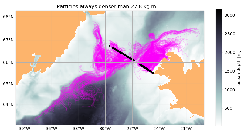
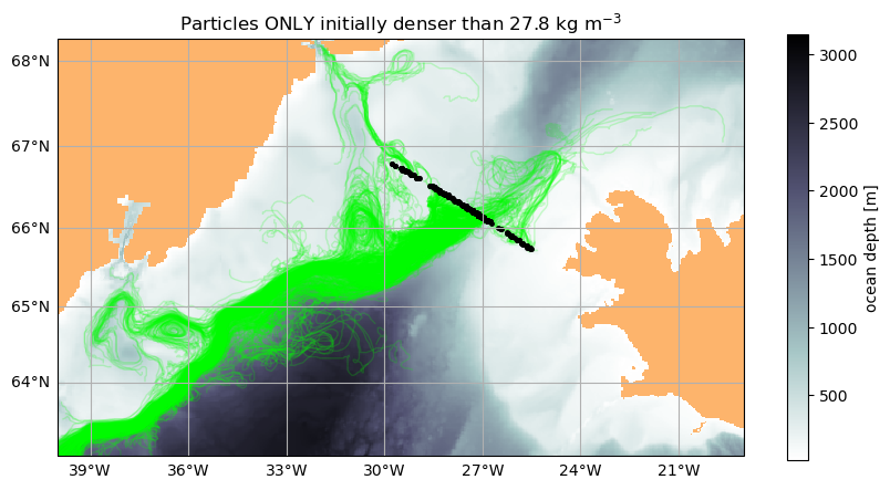
TS-diagrams
We can use TS-diagrams to investigate the hydrographic properties of the od_dense and od_mixed sets. For example, here we plot each oceandataset color-coded by particle depths separately (subplots a and b), then we plot them together on the same isopycnal contours (subplot c).
[12]:
fig = plt.figure(figsize=(10, 10))

for i, (od_i, col, tit) in enumerate(zip(ods, colors, titles)):
    plt.subplot(int("22" + str(i + 1)))
    ax = od_i.plot.TS_diagram(
        colorName="Z", alpha=0.5, cmap_kwargs={"vmin": -2000, "vmax": 0}
    )
    ax.set_title(chr(ord("a") + i) + ") " + tit)

plt.subplot(212)
Tlim = [
    min([od_i.dataset["Temp"].min().values for od_i in ods]),
    max([od_i.dataset["Temp"].max().values for od_i in ods]),
]
Slim = [
    min([od_i.dataset["S"].min().values for od_i in ods]),
    max([od_i.dataset["S"].max().values for od_i in ods]),
]
for i, (od_i, col, tit) in enumerate(zip(ods, colors, titles)):
    contour_kwargs = {}
    if i == 0:
        contour_kwargs["levels"] = []
    ax = od_i.plot.TS_diagram(
        color=col,
        alpha=0.1,
        Tlim=Tlim,
        Slim=Slim,
        contour_kwargs=contour_kwargs,
    )
tit = "\n".join(
    ["c) "] + [f"{col}: {tit}" for _, (col, tit) in enumerate(zip(colors, titles))]
)
ax.set_title(tit)

plt.tight_layout()
Isopycnals: Computing potential density anomaly using the following parameters: {'eq_state': 'jmd95'}.
Isopycnals: Computing potential density anomaly using the following parameters: {'eq_state': 'jmd95'}.
Isopycnals: Computing potential density anomaly using the following parameters: {'eq_state': 'jmd95'}.
Isopycnals: Computing potential density anomaly using the following parameters: {'eq_state': 'jmd95'}.
/home/idies/mambaforge/envs/Oceanography/lib/python3.9/site-packages/oceanspy/plot.py:306: UserWarning: No contour levels were found within the data range.
  CS = ax.contour(s.values, t.values, dens.values, **contour_kwargs)
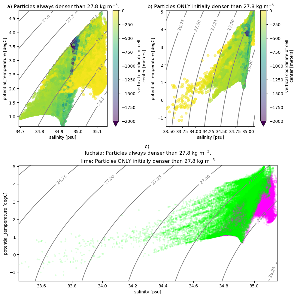
Time series
Now, we select 5 particles that were seeded in the overflow and became less dense along the path using the od_mixed set:
[13]:
nparts = 5
step = np.ceil(len(od_mixed.dataset["particle"]) / 5)
od_5parts = ospy.OceanDataset(
    od_mixed.dataset.isel(particle=slice(None, None, int(step)))
)
Here is a plot of their trajectories:
[14]:
ods = [od_dense, od_mixed]
colors = ["fuchsia", "lime"]
titles = [
    r"Particles always denser than 27.8 kg m$^{-3}$.",
    r"Particles ONLY initially denser than 27.8 kg m$^{-3}$",
]

# Plot Depth
fig = plt.figure(figsize=(10, 5))
ax = od_eul.plot.horizontal_section(varName="masked_Depth", cmap="bone_r")
land_col = (253 / 255, 180 / 255, 108 / 255)
ax.patch.set_facecolor(land_col)
ax.set_extent([-40, -19, 63, 68])

# Plot trajectories
traj = ax.plot(
    od_5parts.dataset["XC"],
    od_5parts.dataset["YC"],
    linewidth=3,
    transform=PlateCarree(),
)

# Plot initial positions
i_pos = ax.plot(
    od_5parts.dataset["XC"].isel(time=0),
    od_5parts.dataset["YC"].isel(time=0),
    "k.",
    markersize=10,
    transform=PlateCarree(),
)
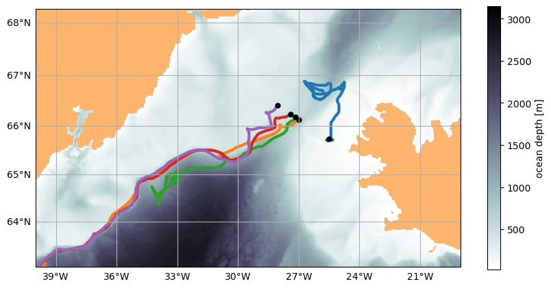
Now we plot the change in potential density anomaly as a function of time of these five particles (1st plot below), and the potential density anomaly gradient (2nd plot). The rapid decrease in particle density corresponds to intense mixing and entrainment of lighter ambient water as the overflow descends into the Irminger Sea. Notice one particle on the Iceland shelf (in blue) is not part of the overflow and moves north then mixes.
[15]:
varName = "Sigma0"
fig, axes = plt.subplots(2, 1, figsize=(10, 10), sharex=True)
for i, ax in enumerate(axes.flatten()):
    if i == 1:
        varName = f"d{varName}_dtime"
    ax = od_5parts.plot.time_series(varName=varName, ax=ax, linewidth=2)
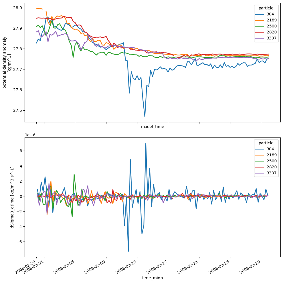
The plots above can be easily customized for any of the extracted variables. For example, change varName = 'Sigma0' in the cell above with any of the variables printed below.
[16]:
# Create table
table = {
    var: od_5parts.dataset[var].attrs.pop(
        "long_name", od_5parts.dataset[var].attrs.pop("description", None)
    )
    for var in od_5parts.dataset.variables
    if "time" not in var and "particle" not in var
}
print("\n{:>15}: {}\n".format("varName", "label"))
for name, desc in sorted(table.items()):
    print("{:>15}: {}".format(name, desc))
        varName: label

          Depth: ocean depth
              S: salinity
         Sigma0: potential density anomaly
           Temp: potential_temperature
             XC: longitude
             XG: longitude
             YC: latitude
             YG: latitude
              Z: vertical coordinate of cell center
             Zl: vertical coordinate of upper cell interface
            Zp1: vertical coordinate of cell interface
             Zu: vertical coordinate of lower cell interface
       momVort3: 3rd component (vertical) of Vorticity