This page was generated from /home/docs/checkouts/readthedocs.org/user_builds/oceanspy/checkouts/latest/docs/Statistics.ipynb.

Use Case 3: Hydrographic Statistics

In this example, we compute some useful hydrographic statistics. We show how to properly account for different grid cell volumes using weighted statistics. The computation is accelerated using dask.

[1]:

# Setup environment:
import matplotlib.pyplot as plt

# Additional packages
import numpy as np
import xarray as xr

import oceanspy as ospy

The following cell starts a dask client (see the Dask Client section in the tutorial).

[2]:

import warnings

import dask

# Start client for multiprocessing
from dask.distributed import Client

client = Client()
client

[2]:

Client

Client-26ae3825-d8e2-11ed-8cff-0242ac110006

Connection method: Cluster object	Cluster type: distributed.LocalCluster
Dashboard: http://127.0.0.1:8787/status

Cluster Info

LocalCluster

81cdac5e

Dashboard: http://127.0.0.1:8787/status	Workers: 4
Total threads: 4	Total memory: 100.00 GiB
Status: running	Using processes: True

Scheduler Info

Scheduler

Scheduler-4d7a9c82-5cdf-4ce7-9c42-615ef58e770e

Comm: tcp://127.0.0.1:44090	Workers: 4
Dashboard: http://127.0.0.1:8787/status	Total threads: 4
Started: Just now	Total memory: 100.00 GiB

Workers

Worker: 0

Comm: tcp://127.0.0.1:35621	Total threads: 1
Dashboard: http://127.0.0.1:40576/status	Memory: 25.00 GiB
Nanny: tcp://127.0.0.1:34369
Local directory: /tmp/dask-worker-space/worker-8_d4bcgx

Worker: 1

Comm: tcp://127.0.0.1:37592	Total threads: 1
Dashboard: http://127.0.0.1:44162/status	Memory: 25.00 GiB
Nanny: tcp://127.0.0.1:40318
Local directory: /tmp/dask-worker-space/worker-2pud10zh

Worker: 2

Comm: tcp://127.0.0.1:34588	Total threads: 1
Dashboard: http://127.0.0.1:35118/status	Memory: 25.00 GiB
Nanny: tcp://127.0.0.1:42551
Local directory: /tmp/dask-worker-space/worker-ccmr530j

Worker: 3

Comm: tcp://127.0.0.1:40062	Total threads: 1
Dashboard: http://127.0.0.1:36471/status	Memory: 25.00 GiB
Nanny: tcp://127.0.0.1:34549
Local directory: /tmp/dask-worker-space/worker-emp51ee1

Open the oceandataset and compute the potential density anomaly:

[3]:

SciServer = True  # True: SciServer - False: any computer
if SciServer:
    od_snapshot = ospy.open_oceandataset.from_catalog("get_started")
else:
    import os

    if not os.path.isdir("oceanspy_get_started"):
        # Download get_started
        import subprocess

        print("Downloading and uncompressing get_started data...")
        print("...it might take a couple of minutes.")
        commands = [
            "wget -v -O oceanspy_get_started.tar.gz -L "
            "https://livejohnshopkins-my.sharepoint.com/"
            ":u:/g/personal/malmans2_jh_edu/"
            "EXjiMbANEHBZhy62oUDjzT4BtoJSW2W0tYtS2qO8_SM5mQ?"
            "download=1",
            "tar xvzf oceanspy_get_started.tar.gz",
            "rm -f oceanspy_get_started.tar.gz",
        ]
        subprocess.call("&&".join(commands), shell=True)
    od_snapshot = ospy.open_oceandataset.from_zarr("oceanspy_get_started")

od_snapshot = od_snapshot.compute.potential_density_anomaly()

Opening get_started.
Small cutout from EGshelfIIseas2km_ASR_crop.
Citation:
 * Almansi et al., 2020 - GRL.
See also:
 * EGshelfIIseas2km_ASR_full: Full domain without variables to close budgets.
 * EGshelfIIseas2km_ASR_crop: Cropped domain with variables to close budgets.
Computing potential density anomaly using the following parameters: {'eq_state': 'jmd95'}.

Make a temperature/salinity diagram.

[4]:

# The statistics are computed using these data.
fig = plt.figure(figsize=(10, 10))
od_snapshot.plot.TS_diagram(markersize=1, alpha=0.5)

# Print number of samples
n_samples = od_snapshot.dataset["Temp"].count().values
print("\nNumber of samples: {:,}\n".format(n_samples))

Isopycnals: Computing potential density anomaly using the following parameters: {'eq_state': 'jmd95'}.

Number of samples: 5,927,388

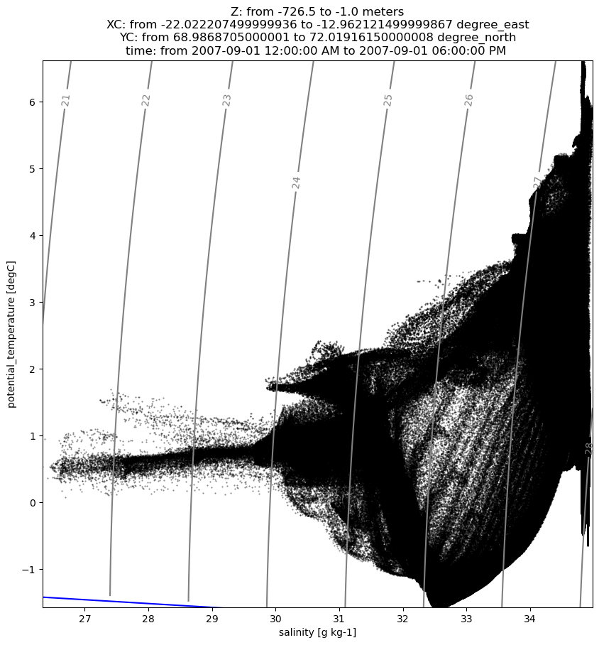
The temperature/salinity diagram shows the distribution of watermass types in terms of their hydrographic properties. Each dot represents a single grid cell in the dataset. We will compute statistics using this data to interpret the plot above.

Binning and Parallelization

We define a function bin_snapshot to perform the binning we need to compute the volume-weighted statistics, or the mode of a variable. The use of the xarray stack method accelerates the groupby_bins task.

[5]:

# Function for binning a single snapshot in time
# dat       = data array to bin (e.g., temperature distributed over 3D space)
# weights   = data array of the relative volumes of the cells in 3D space
# bin_edges = array of the edges of the bins (e.g. temperature bins)
# bin_mid   = array of the mid-points of the bins


def bin_snapshot(dat, weight, bin_edges, bin_mid):
    # Speed up by stacking over space
    dat = dat.stack(alldims=["X", "Y", "Z"])
    weight = weight.stack(alldims=["X", "Y", "Z"])

    # Bin the weight data into these variable bins
    # using the xarray groupby_bins method
    return weight.groupby_bins(
        dat.rename("groups"),
        bins=bin_edges,
        labels=bin_mid,
        include_lowest=True,
    ).sum()

Pick True or False for the parallel variable below to run bin_snapshot with/without dask.

[6]:

# Parallel switch
parallel = True

Raw statistics

First compute and report some raw statistics using xarray, for comparison below. Because we ignore the different volumes of model grid cells, these statistics are not representative of the underlying fields.

[7]:

# Compute and print raw statistics

# Define the percentiles required:
qiles = [0.01, 0.50, 0.99]

# Define the variables required:
var_list = ["Temp", "S", "Sigma0"]

# Pretty print the results:
print("Raw statistics (not volume-weighted):")
print(
    "{:>25s}: {:>10s} {:>10s} {:>10s} {:>10s} {:>10s} {:>10s} {:s}".format(
        "Variable", "mean", "std", "mode", "1", "50", "99", "percentiles"
    )
)

# Loop over variables computing statistics using xarray methods.
# Variables need to be load because dask chunks are not compatible
# with xarray quantiles function.
for var in var_list:
    print("{:25s}:".format(od_snapshot.dataset[var].long_name), end=" ")

    # Data
    dats = getattr(od_snapshot.dataset, var).load()

    # Mean
    var_mean = dats.mean(keep_attrs=True)
    print("{:10.4g}".format(var_mean.values), end=" ")

    # Std
    var_std = dats.std(keep_attrs=True)
    print("{:10.4g}".format(var_std.values), end=" ")

    # Mode
    bin_edges = np.linspace(dats.min(), dats.max(), 512)
    bin_mid = (bin_edges[:-1] + bin_edges[1:]) / 2
    # Parallel switch
    if parallel:
        bin_snapshot_ = dask.delayed(bin_snapshot)

        # Needs to load first
        dat1 = [
            bin_snapshot_(
                dats.sel(time=time).load(),
                xr.ones_like(dats).sel(time=time).load(),
                bin_edges,
                bin_mid,
            )
            for time in dats["time"]
        ]

        with warnings.catch_warnings():
            warnings.simplefilter("ignore")
            dat1 = dask.compute(dat1)[0]
    else:
        dat1 = [
            bin_snapshot(
                dats.sel(time=time),
                xr.ones_like(dats).sel(time=time),
                bin_edges,
                bin_mid,
            )
            for time in dats["time"]
        ]
    dat1 = xr.concat(dat1, "time").sum("time")
    var_mode = dat1["groups_bins"].where(dat1 == dat1.max(), drop=True)
    print("{:10.4g}".format(var_mode.values.squeeze()), end=" ")

    # Qiles
    var_qiles = dats.quantile(qiles, keep_attrs=True)
    print(
        "{:10.4g} {:10.4g} {:10.4g} {:s}".format(
            var_qiles.sel(quantile=qiles[0]).values,
            var_qiles.sel(quantile=qiles[1]).values,
            var_qiles.sel(quantile=qiles[2]).values,
            od_snapshot.dataset[var].units,
        )
    )

    del dats

Raw statistics (not volume-weighted):
                 Variable:       mean        std       mode          1         50         99 percentiles
potential_temperature    :     0.8009      1.366     0.1019     -1.421     0.4803      5.716 degC
salinity                 :      34.44     0.9865       34.9      30.68      34.89      34.93 g kg-1
potential density anomaly:      27.59     0.7954      28.01      24.55      27.97      28.05 kg/m^3

Weighted statistics

Compute the weighted mean (OceanSpy provides a method to do so).

[8]:

od_snapshot = od_snapshot.compute.weighted_mean(varNameList=var_list)

# Print computed variables
print("\nVariables added:")
for var in od_snapshot.dataset.data_vars:
    if any(
        [(var == v or var == f"weight_{v}" or var == f"w_mean_{v}") for v in var_list]
    ):
        print(
            "{:>15}: {} [{}]".format(
                var,
                od_snapshot.dataset[var].long_name,
                od_snapshot.dataset[var].units,
            )
        )

Computing weighted_mean.

Variables added:
           Temp: potential_temperature [degC]
              S: salinity [g kg-1]
         Sigma0: potential density anomaly [kg/m^3]
    w_mean_Temp: potential_temperature [degC]
    weight_Temp: Weights for average [s*m^2*m]
       w_mean_S: salinity [g kg-1]
       weight_S: Weights for average [s*m^2*m]
  w_mean_Sigma0: potential density anomaly [kg/m^3]
  weight_Sigma0: Weights for average [s*m^2*m]

The weights used by OceanSpy have been stored in od_snapshot. The weights correspond to space-time volume elements \(dx \; dy\; dz\; dt\) and hence have units of m\(^3\)s. The variations in the weights are dominated by variations in grid cell volume, which comes from \(dz\) (see below), although \(dx\) and \(dy\) are also important. As the timestep \(dt\) is constant it isn’t responsible for any variation in the weights. We can use the weights, for example, to color a TS-diagrams and better understand which temperature and salinity values are misrepresented using raw statistics.

[9]:

# Scatter plots are not optimized for large amount of samples,
# so the following TS-diagram only shows sea surface water.
fig = plt.figure(figsize=(10, 10))
ax = od_snapshot.plot.TS_diagram(
    s=1,
    alpha=0.5,
    colorName="weight_Temp",
    cutout_kwargs={"ZRange": 0, "dropAxes": True},
)

Cutting out the oceandataset.
Isopycnals: Computing potential density anomaly using the following parameters: {'eq_state': 'jmd95'}.

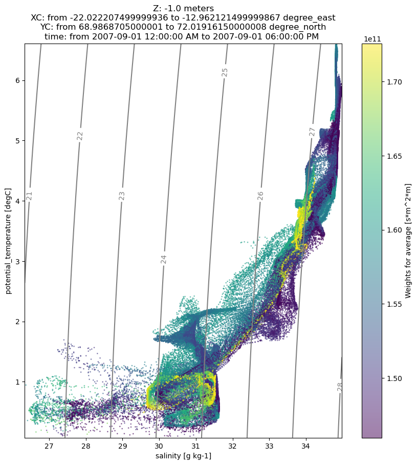
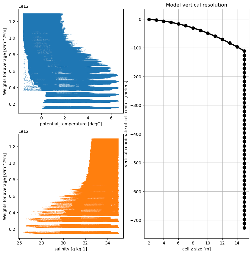
The vertical resolution of the model linearly increases from 1 to 15m in the upper 120m and is 15m thereafter. The following plots show that the weights of warmer and fresher water masses are overestimated in the raw statistics.

[10]:

fig = plt.figure(figsize=(10, 10))

for i, (var, pos) in enumerate(zip(["Temp", "S"], [221, 223])):
    ax = plt.subplot(pos)
    data = od_snapshot.dataset[var]
    weight = od_snapshot.dataset[f"weight_{var}"]
    ax.plot(
        data.values.flatten(),
        weight.values.flatten(),
        ".",
        color=f"C{i}",
        alpha=0.5,
        markersize=0.5,
    )
    ax.set_xlabel(f"{data.long_name} [{data.units}]")
    ax.set_ylabel(f"{weight.long_name} [{weight.units}]")
ax = plt.subplot(122)
drF = od_snapshot.dataset["drF"]
Z = od_snapshot.dataset["Z"]
line = ax.plot(drF, Z, ".-", color="k", linewidth=3, markersize=15)
xlab = ax.set_xlabel(f"{drF.long_name} [{drF.units}]")
ylab = ax.set_ylabel(f"{Z.long_name} [{Z.units}]")
tit = ax.set_title("Model vertical resolution")
ax.grid(True)

Next compute and report the same statistics as before but taking into account the different volumes of different grid cells. We also plot probability distribution and cumulative distribution functions.

[11]:

# Setup plotting
fig, axes = plt.subplots(1, len(var_list), figsize=(30, 10))
hist_color = "tab:red"
qiles_color = "tab:blue"
stat_color = "tab:green"
stat_color2 = "tab:cyan"
stat_color3 = "tab:pink"
stat_color4 = "tab:brown"
bin_edges2 = np.linspace(0, 1, 512)
qiles2 = (bin_edges2[:-1] + bin_edges2[1:]) / 2

# Pretty print the results:
print("Raw statistics (not volume-weighted):")
print(
    "{:>25s}: {:>10s} {:>10s} {:>10s} {:>10s} {:>10s} {:>10s} {:s}".format(
        "Variable", "mean", "std", "mode", "1", "50", "99", "percentiles"
    )
)

# Loop over variables of interest to compute std and percentiles (quantiles),
# pretty print, and plot
for i, (var, ax) in enumerate(zip(var_list, axes.flat)):
    # Print on the way to monitor progress
    var_name = od_snapshot.dataset[var].long_name
    units = od_snapshot.dataset[var].attrs["units"]
    print("{:25s}:".format(var_name), end=" ")

    # Extract variables
    dats = getattr(od_snapshot.dataset, var)
    weights = getattr(od_snapshot.dataset, "weight_" + var)

    # Normalize weights
    weights = weights.where(dats.notnull())
    weightsum = weights.sum()
    weights = weights / weightsum

    # Compute the arithmetic mean
    var_mean = getattr(od_snapshot.dataset, "w_mean_" + var)
    print("{:10.4g}".format(var_mean.values), end=" ")

    # There is no OceanSpy method to compute
    # the weighted standard deviation or percentiles.

    # Compute the standard deviation
    dat2 = ((od_snapshot.dataset[var] - var_mean) ** 2) * weights
    var_std = np.sqrt(dat2.sum().values)
    print("{:10.4g}".format(var_std), end=" ")

    # Define bin edges and mid points for the variable in question.
    # We use 512 uniformly-spaced bins:
    bin_edges = np.linspace(dats.min(), dats.max(), 512)
    bin_mid = (bin_edges[:-1] + bin_edges[1:]) / 2

    # Compute percentiles:
    # Parallel switch
    if parallel:
        bin_snapshot_ = dask.delayed(bin_snapshot)
        # Needs to load first
        dat3 = [
            bin_snapshot_(
                dats.sel(time=time).load(),
                weights.sel(time=time).load(),
                bin_edges,
                bin_mid,
            )
            for time in dats["time"]
        ]
        with warnings.catch_warnings():
            warnings.simplefilter("ignore")
            dat3 = dask.compute(dat3)[0]
    else:
        dat3 = [
            bin_snapshot(
                dats.sel(time=time), weights.sel(time=time), bin_edges, bin_mid
            )
            for time in dats["time"]
        ]

    # Concatenate dat
    dat3 = xr.concat(dat3, "time").sum("time")
    var_hist = dat3 / weights.sum()
    dat4 = dat3.cumsum()
    dat5 = dat4 / weights.sum()

    # Mode
    var_mode = dat3["groups_bins"].where(dat3 == dat3.max(), drop=True)
    print("{:10.4g}".format(var_mode.values.squeeze()), end=" ")

    # Use numpy interpolation to find the percentiles
    # - effectively evaluating the inverse CDF
    var_qiles = np.interp(qiles, dat5, bin_mid)
    var_qiles2 = np.interp(qiles2, dat5, bin_mid)
    var_median = np.interp(0.50, dat5, bin_mid)
    var_limits = np.interp([0.01, 0.99], dat5, bin_mid)
    for var_qile in var_qiles:
        print("{:10.4g}".format(var_qile), end=" ")
    print("{:s}".format(units))

    # Plot the PDF
    p0 = ax.plot(bin_mid, var_hist, "-", color=hist_color, label="PDF", linewidth=4)
    ax.set_xlabel(var_name + " [" + units + "]", fontsize=15)
    ax.set_ylabel("Probability distribution function", fontsize=15, color=hist_color)
    ax.tick_params(axis="y", labelcolor=hist_color)
    ax.grid(True)
    ax.set_xlim(var_limits)

    # Compute and plot the CDF
    ax2 = ax.twinx()
    p1 = ax2.plot(var_qiles2, qiles2, "-", color=qiles_color, label="CDF", linewidth=4)
    ax2.set_ylabel("Cumulative distribution function", fontsize=15, color=qiles_color)
    ax2.tick_params(axis="y", labelcolor=qiles_color)
    ax2.set_xlim(var_limits)

    # Add statistics to plot
    p2 = ax.axvspan(var_mean - var_std, var_mean + var_std, color=stat_color)
    l1 = ax.axvline(var_mean, linestyle="-", color="w", linewidth=2)
    l2 = ax.axvline(var_median, linestyle="--", color=stat_color3, linewidth=2)
    l3 = ax.axvline(var_mode, linestyle="--", color=stat_color4, linewidth=2)
    ax.legend((l2, l3, p2), ("median", "mode", "mean +/- std"), loc="upper left")

Raw statistics (not volume-weighted):
                 Variable:       mean        std       mode          1         50         99 percentiles
potential_temperature    :     0.5422      1.033     0.1019     -1.435     0.3659      4.811 degC
salinity                 :       34.6     0.7318       34.9       31.5      34.89      34.92 g kg-1
potential density anomaly:      27.75     0.5858      28.01      25.24      27.98      28.05 kg/m^3

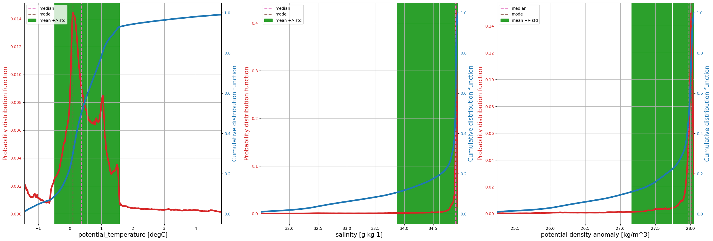
Notice the difference between the weighted mean statistics (in the table of numbers immediately above) and the raw statistics (further above). For example, the weighted-mean temperatures are significantly cooler. The reason is that the grid cell volumes vary, which is ignored in the computation of the raw mean.

Notice how the salinity distribution (probability density function) resembles the potential density anomaly distribution, indicating that density is controlled by salinity, not temperature. This fact is reflected in the T/S diagrams above by the nearly vertical contours of density anomaly. This is a beta-ocean in the parlance of Carmack (2007) and Stewart & Haine (2016).

Notice how the computation is accelerated using dask (try running with/without dask by setting the parallel flag at the top of this notebook).

Volumetric census

A natural extension of these concepts is to compute and plot the volumetric census over temperature/salinity classes. The plots above of probability distribution and cumulative distribution functions focus only on the variable of interest. In other words, the temperature binning to construct the histogram (var_hist in the code) ignores the salinity. But we’re also interested in binning simultaneously into temperature and salinity classes. This quantity is (essentially) the joint distribution function of seawater volume over temperature and salinity.

To compute the joint distribution of volume over temperature and salinity requires two-dimensional binning. This functionality is achieved using the xhistogram package.

[12]:

from xhistogram.xarray import histogram

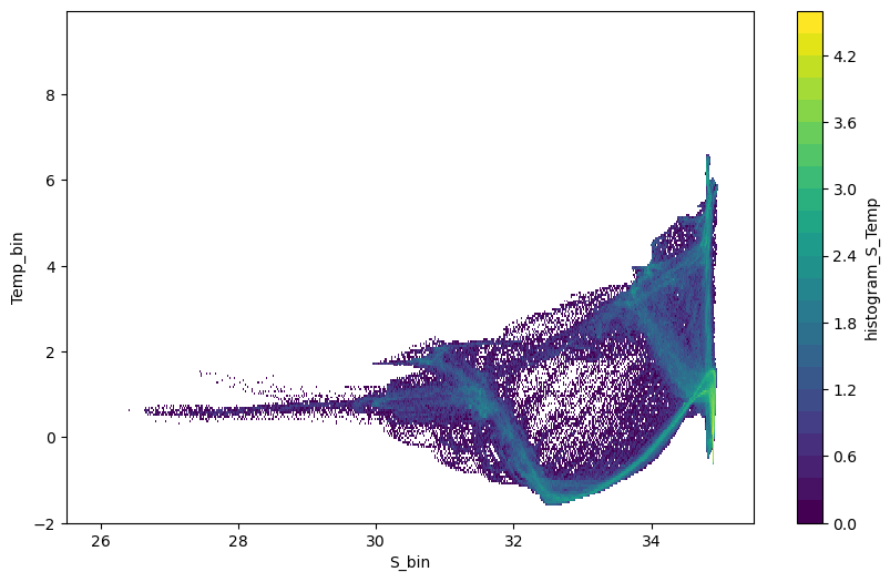
First we construct a histogram of the number of data points in each temperature and salinity class. The temperature and salinity classes are defined using tbins and sbins. All timesteps are considered in the histogram. The colorscale is logarithmic.

[13]:

# Histogram of number of data points. From xhistogram tutorial:
sbins = np.arange(25.5, 35.5, 0.0125)
tbins = np.arange(-2, 10, 0.05)
fig = plt.figure(figsize=(10, 6))
hTS = histogram(
    od_snapshot.dataset["S"].mean("time"),
    od_snapshot.dataset["Temp"].mean("time"),
    bins=[sbins, tbins],
)
np.log10(hTS.T).plot(levels=31)

/home/idies/mambaforge/envs/Oceanography/lib/python3.9/site-packages/dask/core.py:119: RuntimeWarning: divide by zero encountered in log10
  return func(*(_execute_task(a, cache) for a in args))

[13]:

<matplotlib.collections.QuadMesh at 0x7f82773b34f0>

Next we construct the histogram taking into account the different cell volumes. The weight_S variable from compute.weighted_mean supplies these cell volumes (we could also use the weight_T variable). This histogram shows the volume (\(m^3\)) in each temperature and salinity class.

[14]:

# Histogram using volume weights.
dVol = ospy.compute.weighted_mean(
    od_snapshot, varNameList="S", axesList=["X", "Y", "Z"]
)["weight_S"]
fig = plt.figure(figsize=(10, 6))
hTSw = histogram(
    od_snapshot.dataset["S"],
    od_snapshot.dataset["Temp"],
    bins=[sbins, tbins],
    weights=dVol,
)
np.log10(hTSw.T).plot(levels=31)

Computing weighted_mean.

/home/idies/mambaforge/envs/Oceanography/lib/python3.9/site-packages/dask/core.py:119: RuntimeWarning: divide by zero encountered in log10
  return func(*(_execute_task(a, cache) for a in args))

[14]:

<matplotlib.collections.QuadMesh at 0x7f819f416d30>

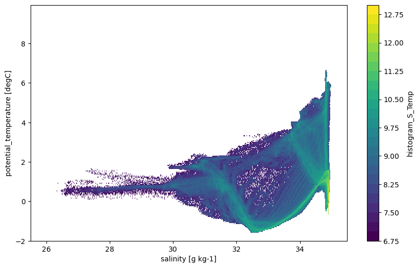
This is the volumetric census over water temperature and salinity classes.